Production patterns of multinational
enterprises: the knowledge-capital model
revisited
著者
Oyamada Kazuhiko
権利
Copyrights 日本貿易振興機構(ジェトロ)アジア
経済研究所 / Institute of Developing
Economies, Japan External Trade Organization
(IDE-JETRO) http://www.ide.go.jp
journal or
publication title
IDE Discussion Paper
volume
674
year
2017-06
INSTITUTE OF DEVELOPING ECONOMIES
IDE Discussion Papers are preliminary materials circulated to stimulate discussions and critical comments
Keywords: foreign direct investment; multinational enterprise; export platform; complex
integration; free trade agreement; economic partnership agreement
JEL classification: F11; F12; F15; F23
IDE DISCUSSION PAPER No. 674
Production Patterns of Multinational Enterprises: The Knowledge-Capital Model Revisited
Kazuhiko OYAMADA July 2017
Abstract
To prepare an answer to the question of how a developing country can attract foreign direct investment (FDI), this paper explored the factors and policies that may help bring FDI into a developing country by utilizing an extended version of the knowledge-capital model. With a special focus on the effects of a free trade agreement (FTA) or an economic partnership agreement (EPA) between a pair of market and non-market countries, simulations with the model revealed the following: (1) although FTA/EPA generally tends to increase FDI to a developing country, the possibility of improving welfare through increased demand for skilled and unskilled labor decreases as the size of the country grows; (2) a developing country may suffer severe welfare losses through FTA/EPA if the availability of skilled labor is extremely limited; and (3) a developing country can enhance welfare gains from a FTA, and it is even possible to recover the welfare effects from negative to positive, by making the arrangement an EPA.
The Institute of Developing Economies (IDE) is a semigovernmental, nonpartisan, nonprofit research institute, founded in 1958. The Institute merged with the Japan External Trade Organization (JETRO) on July 1, 1998.
The Institute conducts basic and comprehensive studies on economic and related affairs in all developing countries and regions, including Asia, the Middle East, Africa, Latin America, Oceania, and Eastern Europe.
The views expressed in this publication are those of the author(s). Publication does not imply endorsement by the Institute of Developing Economies of any of the views expressed within.
INSTITUTE OF DEVELOPING ECONOMIES (IDE), JETRO 3-2-2, WAKABA,MIHAMA-KU,CHIBA-SHI
CHIBA 261-8545, JAPAN
©2017 by Institute of Developing Economies, JETRO
No part of this publication may be reproduced without the prior permission of the IDE-JETRO.
1
Production Patterns of Multinational Enterprises:
The Knowledge-Capital Model Revisited
*Kazuhiko OYAMADA†
July 15, 2017
Abstract
To prepare an answer to the question of how a developing country can attract foreign direct investment (FDI), this paper explored the factors and policies that may help bring FDI into a developing country by utilizing an extended version of the knowledge-capital model. With a special focus on the effects of a free trade agreement (FTA) or an economic partnership agreement (EPA) between a pair of market and non-market countries, simulations with the model revealed the following: (1) although FTA/EPA generally tends to increase FDI to a developing country, the possibility of improving welfare through increased demand for skilled and unskilled labor decreases as the size of the country grows; (2) a developing country may suffer severe welfare losses through FTA/EPA if the availability of skilled labor is extremely limited; and (3) a developing country can enhance welfare gains from a FTA, and it is even possible to recover the welfare effects from negative to positive, by making the arrangement an EPA.
Keywords: foreign direct investment; multinational enterprise; export platform; complex integration; free trade agreement; economic partnership agreement
JEL Classification Numbers: F11; F12; F15; F23
* The author would like to express his gratitude to Michael Ferrantino (World Bank), Ross Hallren (United States International Trade Commission), Elena Ianchovichina (World Bank), David Laborde (International Food Policy Research Institute), Maria Latorre (Universidad Complutense de Madrid), James Markusen (University of Colorado Boulder), Keith Maskus (UC-Boulder), Toshiyuki Matsuura (Keio University), Serge Shikher (USITC), Jacques Thisse (Université Catholique de Louvain), Kazuhiko Yokota (Waseda University), and Wen-Jin Yuan (USITC) for their helpful comments and suggestions.
† Institute of Developing Economies, Japan External Trade Organization (IDE-JETRO), 3-2-2 Wakaba, Mihama-Ku, Chiba-Shi, Chiba 261-8545, Japan ([email protected]).
2
1. Introduction
How can a developing country attract foreign direct investment (FDI)? This question has long been the subject of debate among policy-makers in developing economies, who regard FDI as an important catalyst for economic growth. As the global economy has become increasingly interdependent, multinational enterprises (MNEs) form multilateral production networks, where production processes are subdivided into several stages, and some developing countries have successfully participated in certain parts of these networks. The purpose of this paper is to explore the factors and policies that may help to bring FDI into a developing country.
While research on the activities of MNEs has widely been conducted since the late 1980s, few studies have comprehensively handled every operational pattern of MNEs in one model. In particular, the export-platform is not much discussed in the theoretical studies, even though its importance has been revealed by empirical research. As a low-cost developing country may play a significant role as an export-platform, an analytical model for this study must include this type, in addition to the typical horizontal- and vertical-type MNEs.
One of the most sophisticated studies that consider typical types of MNEs and includes export-platforms in one consistent analytical framework was presented by Ekholm, Forslid, and Markusen (2007). Using a numerical simulation model, in which two market countries and one exogenously given developing country were considered, they explored the conditions under four types of firm strategy, while gradually changing two types of costs, one for trading components and the other for assembling components. However, their model had only one factor of production, and the non-market country was just assumed to set exogenous factor pricing in a partial equilibrium framework. Another work that nests every type of MNE in one model was presented by Ito (2013). Extending the two-region, four-country (two countries in each region) model developed by Navaretti and Venables (2004) to include export-platform, he showed that a reduction in trade costs, either inter-regional or intra-regional, induces firms to choose export-platform, rather than other types. To enable the theoretical model to yield testable hypotheses for empirical testing, he incorporated only trade costs, abstracting production costs away.
A good candidate for the base of an analytical model that includes both trade and production costs in a general equilibrium setting is the knowledge-capital model developed by Markusen (1997), and further extended by Zhang and Markusen (1999). Although export-platform is not taken into account, the computational model can verify effects of
3
changes in firm-type on factor prices in the countries where the MNEs are active. As employment and labor wages in the host country are important factors that MNEs use to decide on a production strategy, this feature based on the general equilibrium nature of the knowledge-capital model is essential for our study. Thus, we utilized an extended version of the model for this study.
The remainder of this paper is organized as follows. Section 2 illustrates the structure and main assumptions of the analytical model. Section 3 explains how the model is parameterized as a numerical model. In Section 4, we perform simulations and report on the results that reveal conditions for which type of firms would be active in a given economic environment, with a special focus on the effects of trade liberalization and optional cost-saving policies. Finally, Section 5 presents the conclusions of this paper.
2. The Extended Knowledge-Capital Model
The model used in this study is a simple extension of the knowledge-capital model that was used as the workhorse in Markusen (2002): we include national enterprises (NEs), horizontal MNEs (HMNEs), vertical MNEs (VMNEs), horizontal export-platforms (HEPs), vertical export-platforms (VEPs), and complexly integrated MNEs (CMNEs). The complex integration strategy, which was introduced by Yeaple (2003) and studied by Grossman, Helpman, and Szeidl (2006), is a combination of the horizontal integration for a foreign market, to reduce trade costs and the vertical export-platform for the home market to reduce production costs. The model is also extended to include two non-market countries, in which the final assembly process of multinational production may take place, while the finished products are not sold locally but exported, in addition to the two market countries assumed in the original model, in which MNEs are established and there are final markets for the commodity produced by those MNEs.1
An important point here is that we do not limit the volumes of those non-market countries, which always stay small in terms of factor endowments. As the knowledge-capital model is a general equilibrium model, branching out and setting up subsidiaries by MNEs in a non-market country affects the local factor prices. If the host country is relatively small, factor prices appreciate more than they would in a relatively
1 While we mainly regard the market and non-market countries in this paper as corresponding to developed and developing countries, respectively, we do not exclude the possibility that a developing country is considered as a market. For example, China could be considered as both final market and non-market production-platform, depending on one's research interest.
4
large country. This may significantly frustrate the incentive of the MNE to stay in the country and trigger it to find another place where cheaper production factors are available. With this model, we investigate which production pattern is adopted by firms established in two countries out of four to sell product in both home and foreign (target) markets under certain economic circumstances.
2.1 Environment
There are four countries: , , , and , indexed as . and are assumed to be countries in which MNEs are established and there are markets for the commodity produced by those MNEs. We index these countries or as a subset of . and are countries in which the final assembly process of multinational productions may take place, while the finished products are not sold locally but exported. The index of these countries is , another subset of .
There are three types of good, , , and . The intermediate good (a component) is used to produce the final product by the MNE. This sector exhibits increasing returns to scale (IRTS), so that the market is assumed to be imperfectly competitive. is produced only in the home of the MNE, country , and is sent to country , where the final assembly process takes place. The finished product is sold on the target market . Note that all MNEs in each production type, national , horizontal , vertical , horizontal export-platform , vertical export-platform , and complex integration , indexed as , share identical technologies and productivities. On the other hand, is the regular good produced by the non-MNE with a constant-returns-to-scale (CRTS) technology so that the market is perfectly competitive. is produced in every country , and sold on the international market as a perfect substitute.
Production factors are of two types, and , which are immobile among national boundaries. Although we mainly regard as skilled labor (human capital) in this study, it can be further extended to include the status of institutions (rules and regulations) and/or the business environment. is unskilled labor. The national endowments of these factors are set exogenously in the model. In the experimental simulations, we change the relative factor endowments for either the market- or non-market-country group, given absolute levels of total endowments for the groups.
In the IRTS sector, two types of fixed costs, and , are required to start operating a firm. Whereas , measured in units of unskilled labor , is needed to set up an assembly plant in country (country specific), , measured in units of skilled labor , is required
5
to establish a firm and its local subsidiary to operate on a trade-link between the home and a foreign country (firm-type/trade-link specific).
There are trade costs (transportation cost and import tariff) for international transport of and , which are specific to each trade link. We assume that unskilled labor in the exporting country is used for the transportation. On the other hand, it is assumed, for simplicity, that shipping does not generate any cost.
2.2 Type-Y Good Producer
There are two groups of firms producing . One is established and headquartered in country , and the other is established and headquartered in country (country ). The markets for are limited to countries and (country ). Good is produced in two stages with IRTS technology by imperfectly competitive firms. In the first stage, each firm produces its components (intermediate good) only in its home country using skilled labor . In the second stage, a firm may send its components to domestic and/or foreign subsidiary(ies) and finalize the production of there, assembling components using locally hired unskilled labor . This assembly process can take place in any country . If the assembly takes place in a non-market country , all of the final products are exported to one or both of the market countries . If it is performed in the home country , the products are sold domestically and/or exported to a foreign market . If it takes place in a foreign market country , the products are sold locally and/or exported back to the home market .
There are both firm-level and plant-level scale economies. By free entry and exit of firms in each operational pattern, a production regime, which refers to a combination of firm-types in an equilibrium, is determined. Following Ekholm, Forslid, and Markusen (2007), regimes will be denoted by suffices with letters, the first letter referring to a firm's home country , the second letter referring to the destination market , and the third letter referring to the location of its assembly plant ( or ). When some of those letters can be omitted without creating any confusion, the length of the suffix becomes shorter. The regimes are categorized into six types, , , , , , and , which express the production pattern of a firm. The six production types are defined as follows.
Type-N: NEs that maintain a single plant with headquarters in country . This type of firms produces both components and final products in country . A fraction of the products may or may not be exported to country .
6
Type-H: HMNEs that maintain plants in both market countries, with headquarters in country . This type of firm produces components in country , some of which are shipped to an assembly plant in country . The final products are produced in both market countries. No fraction of product may be exported.
Type-V: VMNEs that maintain a single plant in the foreign market country , with headquarters in country . This type of firm produces components in country , which are then shipped to the assembly plant in country . A fraction of the products may or may not be exported back to the home market in country .
Type-EH: HEPs that maintain a plant in one of the non-market countries , in addition to a plant and headquarters in home country . This type of firm produces components in country , some of which are shipped to an assembly plant in country . All the final products produced in country are exported to the foreign market in country , while those produced in the home country are sold domestically.
Type-EV: VEPs that maintain a single plant in one of the non-market countries , with headquarters in country . This type of firm produces components in country , which are then shipped to the assembly plant in country . All the final products are exported to both of the market countries .
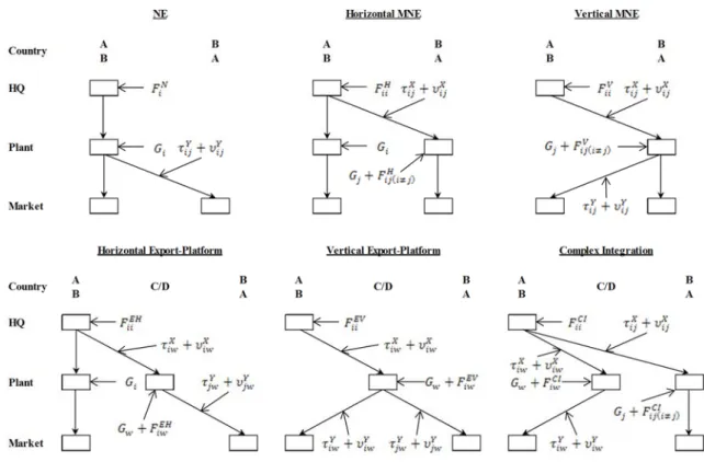
Type-CI: CMNEs that maintain plants both in one of the non-market countries and in the foreign market country , with headquarters in country . This type of firm produces components in country , which are then shipped to the assembly plant in countries and All the final products produced in country are exported back to the home market in country , while those produced in the foreign market country are sold locally. Figure 1 shows schematic images of these six types of production patterns. In each pattern, the headquarters of the firm are located in the country placed on the left-hand side of the image.
7
Figure 1: Six Types of Production Patterns
2.2.1 Type-N Firm Established in Country
The type-N firms produce three kinds of products: components , final products for the domestic market , and final products for the foreign market . The skilled labor requirements to produce one unit of a component in home country can be expressed as:
, (1)
where
is the skilled labor input hired in country ; is the quantity of components produced;
is the fixed cost to establish a NE in country ; and is the unit input requirement for skilled labor.
Similarly, the requirements for both unskilled labor and components to produce one unit of final product in home country can be expressed as:
8
and
∑ , (3)
where
is the unskilled labor hired in country , is the quantity of final products,
is the fixed cost to set up an assembly plant in country , is the unit input requirement for unskilled labor,
is the unit input requirement for components, and
is the rate of transportation margin on final products. Then, the cost function for the type-N firm is given by:
1
, (4)
where
is the price of skilled labor, is the price of unskilled labor, and
is the rate of import tariff on final products.
The first term on the right-hand side of Equation (4) corresponds to the variable costs with respect to . Similarly, the second term corresponds to the variable costs with respect to . The last term corresponds to the total fixed cost.
2.2.2 Type-H Firm Established in Country
The type-H firms produce four kinds of products: components , components , final products for the domestic market , and final products for the foreign market . The skilled labor requirements to produce one unit of components in the home country can be expressed as:
∑ , (5)
where
is the skilled labor input hired in country , is the quantity of components produced, and is the fixed cost to establish a HMNE in country .
9
To ship components from country to destination , the following amount of unskilled labor must be hired in country :
, (6)
where
is the unskilled labor hired for international shipping and is the rate of transportation margin on components.
Next, the requirements for both unskilled labor and components to produce one unit of final products in home country can be expressed as:
(7) and
, (8)
where
is the unskilled labor input hired in country and is the quantity of final products assembled in country .
Similarly, the requirements for both unskilled labor and components to produce one unit of final products in the foreign market country are:
(9)
and
, (10)
where
is the unskilled labor input hired in country ,
is the quantity of final products assembled in country , and is the fixed cost to set up an assembly plant in country .
At the subsidiary in the foreign market country , skilled labor is needed for local administration and management:
, (11)
where
is the skilled labor input hired in country and
is the fixed cost to operate an assembly plant in country . Then, the cost function for the type-H firm is given by:
10
1
∑ , (12)
where
is the rate of import tariff on components.
As in the case of the type-N firm, the first term on the right-hand side of Equation (12) corresponds to the variable cost with respect to . The second term corresponds to those with respect to . The third term is the total fixed cost.
2.2.3 Type-V Firm Established in Country
The type-V firms produce three kinds of products: components , final products for the home market , and final products for the foreign market . The skilled labor requirements to produce one unit of components in the home country can be expressed as:
, (13)
where
is the skilled labor input hired in country , is the quantity of components produced, and is the fixed cost to establish a VMNE in country .
To ship components from country to destination , the following amount of unskilled labor must be hired in country :
, (14)
where
is the unskilled labor hired for international shipping.
Next, the requirements for both unskilled labor and components to produce one unit of final products in the foreign market country can be expressed as:
∑′ ′ (15)
and
∑′ ′ , (16)
where
11
′ is the quantity of final products assembled in country .
Similar to the case of the type-H firm, skilled labor is needed at the subsidiary for local administration and management:
, (17)
where
is the skilled labor input hired in country and
is the fixed cost to operate an assembly plant in country . Then, the cost function for the type-V firm is given by:
1 1
1
∑ ∑ . (18)
Note that ′ ′ 0. The first term on the right-hand side of Equation (18) corresponds
to the variable cost with respect to . The second term corresponds to those with respect to . The third term is the total fixed cost.
2.2.4 Type-EH Firm Established in Country
The type-EH firms produce four kinds of products: components , components , final products for the domestic market , and final products for the foreign market
. The skilled labor requirements to produce one unit of a component in home country can be expressed as:
, (19)
where
is the skilled labor input hired in country ,
is the quantity of components produced for the domestic plant,
is the quantity of components produced for the plant in country , and is the fixed cost to establish a HEP in country .
To ship components from country to a non-market country , the following amount of unskilled labor must be hired in country :
12
, (20)
where
is the unskilled labor hired for international shipping and is the rate of transportation margin on components.
The requirements for both unskilled labor and components to produce one unit of final products in home country can be expressed as:
(21) and
, (22)
where
is the unskilled labor input hired in country and is the quantity of final products assembled in country .
Similarly, the requirements for both unskilled labor and components to produce one unit of final products in non-market country are:
(23) and
, (24)
where
is the unskilled labor input hired in country ,
is the quantity of final products assembled in country for country , is the fixed cost to set up an assembly plant in country , and
is the rate of transportation margin on final products.
At the subsidiary in a non-market country , skilled labor is needed for local administration and management:
, (25)
where
is the skilled labor input hired in country and
is the fixed cost to operate an assembly plant in country . Then, the cost function for the type-EH firm is given by:
1 1
13
where
is the rate of import tariff on final products and is the rate of import tariff on components.
Note that 0 and 0. The correspondence between the expressions on the right-hand side of Equation (26) and the variable or fixed cost is the same as before.
2.2.5 Type-EV Firm Established in Country
The type-EV firms produce two kinds of products: components and final products for market countries . The skilled labor requirements to produce one unit of a component in home country can be expressed as:
, (27)
where
is the skilled labor input hired in country ,
is the quantity of components produced for the plant in country , and is the fixed cost to establish a VEP in country .
To ship components from country to a non-market country , the following amount of unskilled labor must be hired in country :
, (28)
where
is the unskilled labor hired for international shipping.
The requirements for both unskilled labor and components to produce one unit of final product in country can be expressed as:
∑ ∑ (29)
and
∑ , (30)
where
is the unskilled labor input hired in country and
is the quantity of final products assembled in country for country . As in the previous cases, skilled labor is needed at the subsidiary for local administration and management:
, (31)
where
is the skilled labor input hired in country and
14
Then, the cost function for the type-EV firm is given by:
1 1
. (32)
Note that 0. The first term on the right-hand side of Equation (32) corresponds to the variable cost with respect to , and the second term is the total fixed cost.
2.2.6 Type-CI Firm Established in Country
The type-CI firms produce four kinds of products: components , components , final products for the domestic market , and final products for the foreign market . The skilled labor requirements to produce one unit of a component in home country can be expressed as:
, (33)
where
is the skilled labor input hired in country ,
is the quantity of components produced for the plant in country , is the quantity of components produced for the plant in country , and is the fixed cost to establish a CMNE in country .
To ship components and from country to countries and , the following amount of unskilled labor must be hired in country :
, (34)
where
is the unskilled labor hired for international shipping.
The requirements for both unskilled labor and components to produce one unit of final products in the foreign market country can be expressed as:
(35)
and
, (36)
where
is the unskilled labor input hired in country and
is the quantity of final products assembled in country for local sales. Similarly, the requirements for both unskilled labor and components to produce one unit of final products in non-market country are:
15
(37) and
, (38)
where
is the unskilled labor input hired in country and
is the quantity of final products assembled in country for country . At the subsidiaries in countries and , skilled labor is needed for local administration and management, respectively:
(39) and
, (40)
where
is the skilled labor input hired in country ,
is the fixed cost to operate an assembly plant in country , is the skilled labor input hired in country , and
is the fixed cost to operate an assembly plant in country . Then, the cost function for the type-CI firm is given by:
1 1
1
∑ . (41)
Note that 0. The first term on the right-hand side of Equation (41) corresponds to the variable cost with respect to . The second term corresponds to the one with respect to . The rest is the total fixed cost.
2.2.7 Production Volume of a Firm
In an equilibrium, the production volume of a firm in its respective type of production pattern is determined by a pricing relation that assures marginal revenue does not exceed marginal cost. The pricing relations for every type of production pattern can be expressed as:
16 1 1 , (43) 1 ′ 1 ′ ′ 1 ′ ′ ′ ′ ′ ′, (44) 1 , (45) 1 1 1 , (46) 1 1 1 , (47) 1 1 1 , (48) and 1 1 , (49) where
is the price of type-Y good and
is the markup of price over marginal cost ( , , , , , ).
The perpendicular symbol " " shows the complementary slackness relationships between inequalities and endogenous variables. When a relation holds with equality, the corresponding variable takes a positive value.
The optimal markup in a Cournot model with homogeneous products is defined by the firm's share divided by the Marshallian price elasticity of demand in the market. As the Marshallian elasticity of demand is 1 in the present model with Cobb-Douglas demand, a firm's markup can be defined as:
≡ , (50)
where
is the share of type-Y good in the representative consumer's utility function, is an exogenously given level of skilled labor endowment for country , is an exogenously given level of unskilled labor endowment for country , and is tariff revenue in country .
17
Applying (50) to Relations (42) through (49) gives the following:
, (51) , (52) ′ ′ ′ ′ ′ ′ ′ ′ ′, (53) , (54) , (55) , (56) , (57) and . (58)
2.2.8 Number of Firms
Similar to the production volume of a firm, the number of firms in each type of production pattern is determined by a zero-profit condition that assures that markup revenue does not
18
exceed fixed cost payment. The zero-profit conditions for every type of production pattern can be expressed as:
∑ , (59) ∑ ∑ , (60) ∑ ∑′ ′ ′ ′ ∑′ ′ ′ ′ ′ ′ , (61) ∑ , (62) ∑ , (63) and ∑ ∑ ∑ , (64) where
is the number of type-N firms established in country , is the number of type-H firms established in country , is the number of type-V firms established in country ,
is the number of type-EH firms established in country , is the number of type-EV firms established in country , is the number of type-CI firms established in country ,
′ ′ 0,
0, 0, 0, and 0.
Using Relations (42) through (49), and (59) through (64) can be rewritten as:
∑ 1
, (65)
∑ 1 ∑
19 ∑ ∑ 1 ′ ′ 1 ′ ′ ′ ′ ′ ′ ′ ′ ∑′ ′ ′ ′ ′ ′ , (67) ∑ 1 1 , (68) ∑ 1 1 , (69) and 1 1 ∑ 1 ∑ ∑ . (70)
To summarize the type-Y good sector in the model, the output levels and number of firms categorized in the six types of production patterns are determined by Inequalities (51) through (58) and (65) through (70), respectively, given the factor and commodity prices determined by the market-clearing conditions that will be seen later.
2.3 Type-Z Good Producer
The type-Z good is produced in every country with skilled and unskilled labor using a Cobb-Douglas CRTS technology under perfect competition. The production function is:
, (71)
where
is the output volume of type- good in country , is the skilled labor input,
is the unskilled labor input, is the share of skilled labor, and is a scaling factor of measuring units.
20
The producer in every country chooses the levels of , , and , to maximize profit subject to (71), given the prices of skilled and unskilled labor, and , and the output . The first order conditions (FOCs) for the optimum are given by:
(72)
and
1 . (73)
Equations (71) through (73) determine the levels of , , and .
2.4 Consumer
The representative consumer in every country maximizes her/his utility subject to the budget constraint, given the price of commodities.
2.4.1 Consumer in Country
The welfare level of a representative consumer in a market country is assumed to be given by the following Cobb-Douglas utility function:
, (74)
where
is the welfare level of the representative consumer in country , is the consumption level of type-Y good produced in the IRTS sector, is the consumption level of type-Z good produced in the CRTS sector, is the share of type-Y good (mentioned in Subsection 2.2.7), and is a scaling factor.
The budget constraint for the consumer is expressed as:
, (75)
where the expenditure enters the left-hand side, while the budget is sourced by factor income, and tariff revenue appears in the right-hand side of Equation (75). Note that we implicitly assume balanced trade, so there are no foreign savings.
The representative consumer in country chooses the consumption levels of and to maximize her/his utility, defined by Equation (74), subject to (75). The FOCs for the optimum are:
21
(76) and
1 , (77)
where is the Lagrange multiplier with respect to budget constraint (75), which shows the marginal utility of income. Equations (76) and (77) determine the levels of and
.
2.4.2 Consumer in Country
As the type-Y good is sold only in the market countries, the welfare level of the representative consumer in non-market country is measured solely by the consumption level of the type-Z good, as follows:
, (78)
where
is the welfare level of the representative consumer in country and is the consumption level of type-Z good produced in the CRTS sector.
Similar to the previous case, the budget constraint equates expenditure with factor income and tariff revenue, as follows:
. (79)
Again, balanced trade is assumed.
The representative consumer in country chooses the consumption level of to maximize her/his utility, as defined by Equation (78), subject to (79). The FOC for the optimum is:
1, (80)
where is the Lagrange multiplier with respect to budget constraint (79). Equation (80) determines the level of .
2.4.3 Tariff Revenue
The tariff revenues in countries and , respectively, are defined as follows: ≡ ∑
22 ∑ ∑ 1 ∑ ∑′ ′ ∑ ∑ 1 ∑ ∑ 1 ∑ 1 ∑ ∑ and ≡ ∑ ∑ ∑ ∑ ∑ .
We presume that the tariff revenue in each country is transferred to the representative consumer.
2.5 Market Equilibrium
The market-clearing conditions determine the price levels of the corresponding production factors and commodities in an equilibrium.
2.5.1 Factor Market Clearing
In each market country , the following two labor market-clearing conditions hold in an equilibrium:
23 ∑ ∑ ∑ ∑ ∑ (81) and ∑ ∑ ∑ ∑ ∑ ∑ . (82)
Equations (81) and (82), respectively, determine the levels of factor prices and . In each non-market country , the following two market-clearing conditions hold in an equilibrium:
∑ ∑ ∑ (83)
and
∑ ∑ ∑ . (84)
The price levels of skilled and unskilled labor in country , and , are determined by Equations (83) and (84).
2.5.2 Commodity Market Clearing
The demand and supply of the two kinds of commodity for final consumption are equated to determine their price levels, as follows:
∑ ∑′ ′ ′ ∑
∑ ∑
∑ ∑ (85)
and
∑ ∑ . (86)
Equations (85) and (86) determine the price levels of both type-Y and type-Z goods, and .
24
because of Walras' Law, we drop Equation (86) from the system, treating the type-Z good as the numéraire. Consequently, is set to unity, given exogenously.
2.6 System Equations/Inequalities
In the model, the output volumes of the type-Y good in each of the six types of production pattern ( , , ′, , , , , and ), number of firms in the six
types of production pattern ( , , , , , and ), the output volume of the type-Z good ( ), the input volume of skilled and unskilled labor in the production of the type-Z good ( and ), the marginal utility of income for the representative consumer in country ( ), the consumption levels of the two kinds of commodity by the representative consumer in country ( and ), the marginal utility of income for the representative consumer in country ( ), the consumption/welfare level of the type-Z good by the representative consumer in country ( ), the price levels of skilled and unskilled labor in country ( and ), the price levels of the two kinds of labor in country ( and ), and the price level of the type-Y good ( ) are determined by Inequalities (51) through (58) and (65) through (70), and by Equations (71) through (73), (75) through (77), (79), (80), (81) through (84), and (85), respectively.
3. Numerical Implementation of the Model
Markusen (2002) noted that one may face two kinds of computational difficulty in the numerical application of an analytical model such as the one we introduced in the previous section. One difficulty is due to the high-dimensionality of the model, and the other is brought by the handling of inequalities. Versions of the knowledge-capital model, an objective of which is to analyze emerging patterns of independent firm-types under different economic conditions, require us to appropriately manage corner-solutions based on the Karush-Kuhn-Tucker conditions. For this reason, the model used in this study was coded in the General Algebraic Modeling System (GAMS) and solved by its PATH solver, which enables us to easily handle complementary slackness.2
In experimental simulations, we change the relative factor endowments for either the
25
market- or non-market-country groups, given absolute levels of total endowments for the group. The factor endowments for the group that is not being focused on are kept identical for the two countries in the group to avoid complexities in interpreting the results. Then, a box diagram à la Edgeworth box is drawn, placing the total skilled labor endowment for the focused group on one axis and the total unskilled labor endowment on another axis to capture the regime, welfare level, factor prices, etc., in each cell corresponding to the relative factor endowments of the two countries.
The model is calibrated to the center of the box diagram, where the two countries in each group are identical. At this point, it is assumed that only HMNEs are active, due to the existence of high trade costs between the two market countries in the base case. Then, there are no local subsidiaries and plants in the non-market countries, and there is no trade with respect to the type-Z good. Calibration of the model requires a set of information that includes a social accounting matrix (SAM), which corresponds to the center of the box diagram, levels of fixed and trade costs (transportation cost and import tariff), and input coefficients. In particular, careful setting of the firm-type/trade-link specific fixed cost is required, because simulation results tend to be sensitive to this setting, in addition to the fact that the firm-types, other than the type-H, do not enter the given SAM.
3.1 Setting of the Firm-Type/Trade-Link Specific Fixed Cost
Let us recall the three important assumptions for the knowledge-capital model defined by Markusen (2002:129):
Fragmentation: the location of knowledge-based assets may be fragmented from
production. Any incremental cost of supplying services of the asset to a single foreign plant versus the cost to a single domestic plant is small.
Skilled-labor Intensity: knowledge-based assets are skilled labor intensive relative to final
production.
Jointness: the services of knowledge-based assets are (at least partially) joint ("public")
inputs into multiple production facilities. The added cost of a second plant is small compared to the cost of establishing a firm with local plant.
26
three properties, because a firm's decisions to choose between operational types under a certain economic condition are crucially motivated by these properties.
Based on the three properties, we make the following four assumptions on the firm-type/trade-link specific fixed cost for a firm established in country :
2 , (87)
, (88)
, (89)
and
. (90)
The case for a firm established in country is similar. Relation (87) is based on the jointness assumption shown above.
Relation (88) is related to the headquarter cost. First, the type-H firm is more costly than the type-N firm because additional skilled labor is required in the headquarters for managerial and coordination activities. Second, the additional cost of managerial and coordination activities for the operation of a local subsidiary might be higher in a non-market country (type-EH and type-CI) than in a market country (type-H). A similar relation applies to the type-V and type-EV firms. Third, the type-N firm is costlier than either the type-V or type-EV firms, because the latter may hire local skilled labor to train unskilled labor in the host country.
Relation (89) is related to the affiliate cost of local administration and management. In non-market countries, cheaper skilled labor is available.
Relation (90) is related to the total cost. The type-V and type-EV firms are less costly than the type-H and type-EH firms, because the former has only one assembly plant in a non-market country and, thus, additional payment for managerial and coordination activities is not required. Among the type-H and type-EH firms, we assume that operating an assembly plant is costlier in a market country than in a non-market country. A similar relation applies to the type-V and type-EV firms. The costliest firm is the type-CI, because this type operates its headquarters and two assembly plants in three different countries. Relation (90) also implies that technology transfer incurs some amount of cost, so fragmentation is not perfect.
One point to note is that we presume the plant-level production of the type-Y good is less skilled-labor intensive than is that of the type-Z, which represents the composite of all kinds of other commodities, unlike the original theory (Carr, Markusen, and Maskus
27
2001:694; Markusen 2002:133). Based on the Global Trade Analysis Project (GTAP) 9A Data Base for 2011 (Hertel 1997), shares of skilled-labor in the total labor inputs with respect to the manufacturing sector and the sector that includes both primary industries and services in the 24 countries, in which the world's top 100 non-financial MNEs for 2015 (UNCTAD 2016) are established, are 37.837% and 56.795%, respectively, whereas the share with respect to the overall production in the rest of the world is 48.707%.3 The
countries with the top 100 investors can be regarded as the market countries in this study, while the countries without are the non-market countries. Thus, assuming that MNEs mainly reside in the manufacturing sector, we stipulate the skilled-labor intensity of activities as
(Headquarters Only)
(Integrated Production of Type-Y) (Production of Type-Z)
(Plant Only).
This assumption of factor-intensity significantly affects the simulation results, as will be seen later. While MNEs are often considered as being more skilled-labor intensive than are local firms in developing countries, we suspect that the hypothesis holds only for industries classified within the same category. In addition, there has long been debate over whether FDI may substantially increase the wage skill premium. As yet, there is no clear answer to this question (Verhoogen 2008; Amiti and Cameron 2012). Thus, we just set an assumption based on available data and perform simulation experiments.
Finally, the parameter values for the firm-type/trade-link specific fixed cost are set as follows: 4.0, 4.2 , 1.4 , 3.4 , 1.4 , 4.2 , 0 , 1.3 , 3.4 , 0 , 1.3 , and
3 The 24 countries are: Australia, China, Hong Kong, Japan, Korea, Taiwan, Malaysia, United States, Mexico, Brazil, Belgium, Denmark, France, Germany, Ireland, Italy, Luxembourg, Netherlands, Spain, Sweden, United Kingdom, Switzerland, Norway, and Israel. If we also include the top 100 investors from developing and transition economies, 12 countries are added to the previous 24. Those are the Philippines, Singapore, Thailand, India, Argentina, Venezuela, Russian Federation, Kuwait, Qatar, Saudi Arabia, United Arab Emirates, and South Africa. While Algeria should also be included, it is not separately available in the GTAP 9A Data Base. In the latter case, shares of skilled-labor with respect to the three sectors become 37.316%, 56.385%, and 48.616%, respectively. Hence, the ranking of skilled-labor intensity of activities does not change.
28
4.2 , 1.4 , 1.3 .
These values tend to be set high to perform comparative statics between the base case and a counterfactual equilibrium, where some of the values are set substantially lower.
3.2 Calibration Based on a Social Accounting Matrix
Along with the firm-type/trade-link specific fixed cost, transportation cost and import tariff related to the two types of commodity, intermediate and final goods and input coefficients are assumed as follows:
0.1, 0.2, 1,
0.875, and 0.125.
In addition, initial levels of prices are given, as follows, as a usual cliché in the parameterization process of a general equilibrium model, in which not absolute but only relative levels of prices matter:
1 and 1.25.
Then, the initial values of some endogenous variables and a part of the country specific setup cost are calibrated from a SAM. In this study, we assume the following value is obtained from a SAM.
101.0145373.
In the second step, the initial values of is calculated using Equation (52):
16.1623 , 13.5764 .
Third, is derived using the following relation:
∑
.
. . . 2.71738945 ⋯.
is also obtained by Equation (50):
0.2 , 0.168 .
Finally, is calibrated using Equation (66), because the two market countries are identical:
0.6458.
Based on this calibrated value, is also set to 0.6458 in the base case.
29
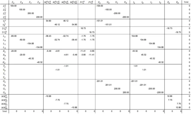
, , , , , and denote total cost, consumption, markup revenue, fixed cost, income of a representative consumer, and income of the type-H firm's owner, respectively. In this case, we presume that all four countries have the same amount of factor endowments. In the later simulation experiments, we will consider different country sizes for the non-market group.
Using this SAM, the parameters in the two Cobb-Douglas aggregator functions (71) and (74), , , , and , are calibrated.
Table 1: Social Accounting Matrix for the Center of the Box Diagram
4. Simulations
We now report on the results of simulations performed with the extended knowledge-capital model introduced previously. The simulations are categorized into two groups. The first grouping is done to reveal some of the behavioral characteristics of the model. The second is done to examine whether a free trade agreement (FTA) or an economic partnership agreement (EPA) would be effective for a non-market (developing) country to stimulate incoming FDI, in a situation where the country is left behind another non-market (developing) rival in forming a free trade area with one of the market countries.
30
In the simulations, we change the relative factor endowments for either the market- or non-market-country group, given absolute levels of total endowments for the group, and we calculate every equilibrium of the economy under the selected sets of national endowments. The factor endowments for the group not under focus are kept identical to two the members in the group. Then, trade and fixed costs, respectively, are reduced from their initial values, set in the base case, to see how the pattern of regimes changes.
4.1 Basic Characteristics of the Model
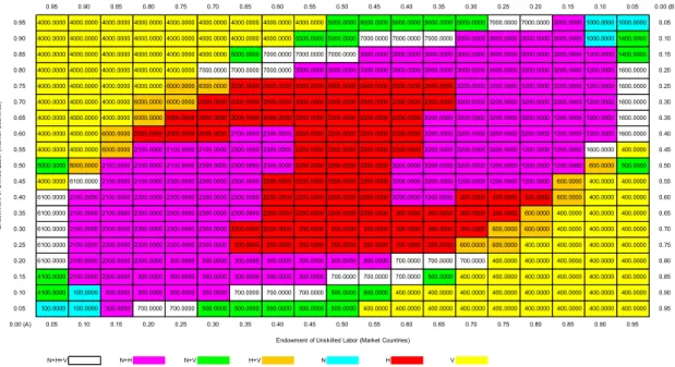
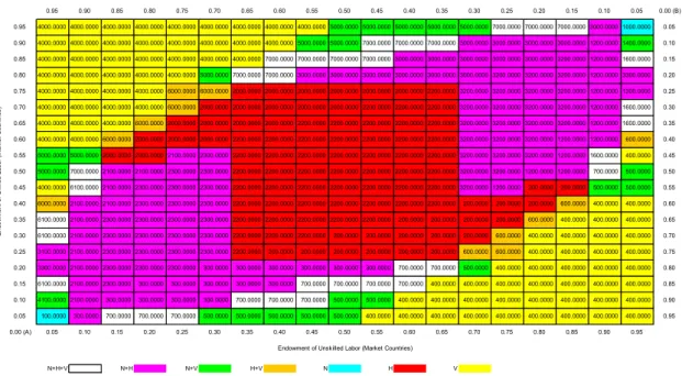
Figure 2: Equilibrium Regime in the Base Case (Market Countries)
Figure 2 is a box diagram for the case when relative factor endowments for the market countries are changed, given the absolute levels of total endowments shown in the benchmark SAM (Table 1). This will be the base case for comparison with the results obtained when a set of parameters or exogenous variables are changed. The initial levels of trade and fixed costs assumed in the base case are:
0.1, 0.2, 4.0, 4.2 , 1.4 , 0.95 0.90 0.85 0.80 0.75 0.70 0.65 0.60 0.55 0.50 0.45 0.40 0.35 0.30 0.25 0.20 0.15 0.10 0.05 0.00 (B) 0.95 4000.0000 4000.0000 4000.0000 4000.0000 4000.0000 4000.0000 4000.0000 4000.0000 4000.0000 5000.0000 5000.0000 5000.0000 5000.0000 5000.0000 7000.0000 7000.0000 3000.0000 1000.0000 1000.0000 0.05 0.90 4000.0000 4000.0000 4000.0000 4000.0000 4000.0000 4000.0000 4000.0000 4000.0000 5000.0000 5000.0000 7000.0000 7000.0000 7000.0000 3000.0000 3000.0000 3000.0000 3000.0000 1000.0000 1400.0000 0.10 0.85 4000.0000 4000.0000 4000.0000 4000.0000 4000.0000 4000.0000 5000.0000 7000.0000 7000.0000 7000.0000 3000.0000 3000.0000 3000.0000 3000.0000 3000.0000 3000.0000 3200.0000 1200.0000 1400.0000 0.15 0.80 4000.0000 4000.0000 4000.0000 4000.0000 4000.0000 7000.0000 7000.0000 7000.0000 3000.0000 3000.0000 3000.0000 3000.0000 3000.0000 3000.0000 3000.0000 3200.0000 3200.0000 1200.0000 1600.0000 0.20 0.75 4000.0000 4000.0000 4000.0000 4000.0000 6000.0000 6000.0000 2000.0000 2000.0000 2000.0000 2000.0000 2000.0000 2000.0000 2000.0000 3200.0000 3200.0000 3200.0000 3200.0000 1200.0000 1600.0000 0.25 0.70 4000.0000 4000.0000 4000.0000 6000.0000 6000.0000 2000.0000 2000.0000 2000.0000 2000.0000 2000.0000 2000.0000 2200.0000 2200.0000 3200.0000 3200.0000 3200.0000 3200.0000 1200.0000 1600.0000 0.30 0.65 4000.0000 4000.0000 4000.0000 6000.0000 2000.0000 2000.0000 2000.0000 2000.0000 2200.0000 2200.0000 2200.0000 2200.0000 3200.0000 3200.0000 3200.0000 3200.0000 1200.0000 1200.0000 1600.0000 0.35 0.60 4000.0000 4000.0000 6000.0000 2000.0000 2000.0000 2000.0000 2100.0000 2300.0000 2200.0000 2200.0000 2200.0000 2200.0000 3200.0000 3200.0000 3200.0000 3200.0000 1200.0000 1200.0000 1600.0000 0.40 0.55 4000.0000 4000.0000 6000.0000 2100.0000 2100.0000 2100.0000 2300.0000 2300.0000 2200.0000 2200.0000 2200.0000 2200.0000 3200.0000 3200.0000 3200.0000 1200.0000 1200.0000 1600.0000 400.0000 0.45 0.50 5000.0000 6000.0000 2100.0000 2100.0000 2100.0000 2300.0000 2300.0000 2300.0000 2200.0000 2200.0000 2200.0000 3200.0000 3200.0000 3200.0000 1200.0000 1200.0000 1200.0000 600.0000 500.0000 0.50 0.45 4000.0000 6100.0000 2100.0000 2100.0000 2300.0000 2300.0000 2300.0000 2200.0000 2200.0000 2200.0000 2200.0000 3200.0000 3200.0000 1200.0000 1200.0000 1200.0000 600.0000 400.0000 400.0000 0.55 0.40 6100.0000 2100.0000 2100.0000 2300.0000 2300.0000 2300.0000 2300.0000 2200.0000 2200.0000 2200.0000 2200.0000 3200.0000 1200.0000 200.0000 200.0000 200.0000 600.0000 400.0000 400.0000 0.60 0.35 6100.0000 2100.0000 2100.0000 2300.0000 2300.0000 2300.0000 2300.0000 2200.0000 2200.0000 2200.0000 2200.0000 200.0000 200.0000 200.0000 200.0000 600.0000 400.0000 400.0000 400.0000 0.65 0.30 6100.0000 2100.0000 2300.0000 2300.0000 2300.0000 2300.0000 2200.0000 2200.0000 200.0000 200.0000 200.0000 200.0000 200.0000 200.0000 600.0000 600.0000 400.0000 400.0000 400.0000 0.70 0.25 6100.0000 2100.0000 2300.0000 2300.0000 2300.0000 2300.0000 200.0000 200.0000 200.0000 200.0000 200.0000 200.0000 200.0000 600.0000 600.0000 400.0000 400.0000 400.0000 400.0000 0.75 0.20 6100.0000 2100.0000 2300.0000 2300.0000 300.0000 300.0000 300.0000 300.0000 300.0000 300.0000 300.0000 700.0000 700.0000 700.0000 400.0000 400.0000 400.0000 400.0000 400.0000 0.80 0.15 4100.0000 2100.0000 2300.0000 300.0000 300.0000 300.0000 300.0000 300.0000 300.0000 700.0000 700.0000 700.0000 500.0000 400.0000 400.0000 400.0000 400.0000 400.0000 400.0000 0.85 0.10 4100.0000 100.0000 300.0000 300.0000 300.0000 300.0000 700.0000 700.0000 700.0000 500.0000 500.0000 400.0000 400.0000 400.0000 400.0000 400.0000 400.0000 400.0000 400.0000 0.90 0.05 100.0000 100.0000 300.0000 700.0000 700.0000 500.0000 500.0000 500.0000 500.0000 500.0000 400.0000 400.0000 400.0000 400.0000 400.0000 400.0000 400.0000 400.0000 400.0000 0.95 0.00 (A) 0.05 0.10 0.15 0.20 0.25 0.30 0.35 0.40 0.45 0.50 0.55 0.60 0.65 0.70 0.75 0.80 0.85 0.90 0.95 N+H+V N+H N+V H+V N H V En do w m en t o f Ski lle d L ab or ( M ar ke t C ou nt rie s)
31 3.4 , 1.4 , 4.2 , 0 , 1.3 , 3.4 , 0 , 1.3 , 4.2 , 1.4 , 1.3 , and 0.6458.
In the box, the vertical axis corresponds to the total endowment of skilled labor for the two market countries, and the horizontal axis corresponds to that of unskilled labor. The division of the factor endowments between the two countries is shown, with country measured from the southwest (SW) corner and country measured from the northeast (NE) corner. The model is repeatedly solved for each cell 361 (19 19) times, altering the distribution of factor endowments. Each cell represents an equilibrium regime, and the number inside shows which type of firm is active in the regime. The regime number is defined as:
,
where
1000 if type-N firms established in country are active, otherwise 0, 100 if type-N firms established in country are active, otherwise 0, 2000 if type-H firms established in country are active, otherwise 0, 200 if type-H firms established in country are active, otherwise 0, 4000 if type-V firms established in country are active, otherwise 0, 400 if type-V firms established in country are active, otherwise 0,
10 if type-EH firms established in country operating in country are active, otherwise 0,
20 if type-EH firms established in country operating in country are active, otherwise 0,
1 if type-EH firms established in country operating in country are active, otherwise 0,
2 if type-EH firms established in country operating in country are active, otherwise 0,
0.1 if type-EV firms established in country operating in country are active, otherwise 0,
0.2 if type-EV firms established in country operating in country are active, otherwise 0,
32
are active, otherwise 0,
0.02 if type-EV firms established in country operating in country are active, otherwise 0,
0.001 if type-CI firms established in country operating in country are active, otherwise 0,
0.002 if type-CI firms established in country operating in country are active, otherwise 0,
0.0001 if type-CI firms established in country operating in country are active, otherwise 0, and
0.0002 if type-CI firms established in country operating in country are active, otherwise 0.
Figure 2 shows that the type-H firms prevail around the center of the box diagram, where two market countries are similar in both size and relative endowment. If the countries are different in size, while being similar in relative endowment, the type-N firms established in the country with abundant factors dominate the production and occupy both markets, as confirmed around the SW and NE corners. When the price of unskilled labor in a market country becomes cheaper, the foreign type-H firms become active in the country, as confirmed in the northwest (NW) and southeast (SE) neighborhoods surrounding the central area. Toward the NW corner from the center, the price of skilled/unskilled labor in country becomes lower/higher while that in country follows the opposite pattern. These relationships reverse toward the SE corner. Thus, firms in a market country where the price of unskilled labor becomes extremely high, go out to the other market country as type-V firms, as confirmed around the NW and SE corners.
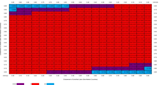
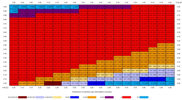
Figure 3 is a box diagram for the case when relative factor endowments for the non-market countries are changed and the absolute levels of total endowments for the group are given. This is also the base case. Figure 3 shows that, along the diagonal between the SW and NE corners, where non-market countries are similar in relative endowment, MNEs never set up plants in non-market countries but go straight to the market countries as type-H firms. This occurs because there is no significant difference between relative factor prices among the countries. On the other hand, around the NW and SE corners, where cheaper unskilled labor is available in either of the non-market countries, the type-EV firms become active. For instance, around the SE corner, unskilled labor is relatively abundant in country , so the type-EV firms from both countries and operate in . Around the NW corner, firms operating in country will be dominant. Note that, in this base case captured by Figures 2 and 3, the type-EH and type-CI firms never show up.
33
Figure 3: Equilibrium Regime in the Base Case (Non-Market Countries)
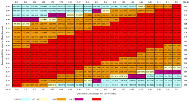
Figure 4: Lower Transportation Cost of Components ( 0, Market Countries)
Next, let us see what happens when selected values of trade and fixed costs change.
0.95 0.90 0.85 0.80 0.75 0.70 0.65 0.60 0.55 0.50 0.45 0.40 0.35 0.30 0.25 0.20 0.15 0.10 0.05 0.00 (D) 0.95 0.2200 0.2200 0.2200 0.2200 0.2200 0.2200 0.2200 0.2200 2200.2200 2200.2200 2200.2200 2200.2200 2200.2200 2200.2200 2200.0000 2200.0000 2200.0000 2200.0000 2200.0000 0.05 0.90 0.2200 2200.2200 2200.2200 2200.2200 2200.2200 2200.2200 2200.2200 2200.2200 2200.0000 2200.0000 2200.0000 2200.0000 2200.0000 2200.0000 2200.0000 2200.0000 2200.0000 2200.0000 2200.0000 0.10 0.85 2200.2200 2200.2200 2200.2200 2200.0000 2200.0000 2200.0000 2200.0000 2200.0000 2200.0000 2200.0000 2200.0000 2200.0000 2200.0000 2200.0000 2200.0000 2200.0000 2200.0000 2200.0000 2200.0000 0.15 0.80 2200.0000 2200.0000 2200.0000 2200.0000 2200.0000 2200.0000 2200.0000 2200.0000 2200.0000 2200.0000 2200.0000 2200.0000 2200.0000 2200.0000 2200.0000 2200.0000 2200.0000 2200.0000 2200.0000 0.20 0.75 2200.0000 2200.0000 2200.0000 2200.0000 2200.0000 2200.0000 2200.0000 2200.0000 2200.0000 2200.0000 2200.0000 2200.0000 2200.0000 2200.0000 2200.0000 2200.0000 2200.0000 2200.0000 2200.0000 0.25 0.70 2200.0000 2200.0000 2200.0000 2200.0000 2200.0000 2200.0000 2200.0000 2200.0000 2200.0000 2200.0000 2200.0000 2200.0000 2200.0000 2200.0000 2200.0000 2200.0000 2200.0000 2200.0000 2200.0000 0.30 0.65 2200.0000 2200.0000 2200.0000 2200.0000 2200.0000 2200.0000 2200.0000 2200.0000 2200.0000 2200.0000 2200.0000 2200.0000 2200.0000 2200.0000 2200.0000 2200.0000 2200.0000 2200.0000 2200.0000 0.35 0.60 2200.0000 2200.0000 2200.0000 2200.0000 2200.0000 2200.0000 2200.0000 2200.0000 2200.0000 2200.0000 2200.0000 2200.0000 2200.0000 2200.0000 2200.0000 2200.0000 2200.0000 2200.0000 2200.0000 0.40 0.55 2200.0000 2200.0000 2200.0000 2200.0000 2200.0000 2200.0000 2200.0000 2200.0000 2200.0000 2200.0000 2200.0000 2200.0000 2200.0000 2200.0000 2200.0000 2200.0000 2200.0000 2200.0000 2200.0000 0.45 0.50 2200.0000 2200.0000 2200.0000 2200.0000 2200.0000 2200.0000 2200.0000 2200.0000 2200.0000 2200.0000 2200.0000 2200.0000 2200.0000 2200.0000 2200.0000 2200.0000 2200.0000 2200.0000 2200.0000 0.50 0.45 2200.0000 2200.0000 2200.0000 2200.0000 2200.0000 2200.0000 2200.0000 2200.0000 2200.0000 2200.0000 2200.0000 2200.0000 2200.0000 2200.0000 2200.0000 2200.0000 2200.0000 2200.0000 2200.0000 0.55 0.40 2200.0000 2200.0000 2200.0000 2200.0000 2200.0000 2200.0000 2200.0000 2200.0000 2200.0000 2200.0000 2200.0000 2200.0000 2200.0000 2200.0000 2200.0000 2200.0000 2200.0000 2200.0000 2200.0000 0.60 0.35 2200.0000 2200.0000 2200.0000 2200.0000 2200.0000 2200.0000 2200.0000 2200.0000 2200.0000 2200.0000 2200.0000 2200.0000 2200.0000 2200.0000 2200.0000 2200.0000 2200.0000 2200.0000 2200.0000 0.65 0.30 2200.0000 2200.0000 2200.0000 2200.0000 2200.0000 2200.0000 2200.0000 2200.0000 2200.0000 2200.0000 2200.0000 2200.0000 2200.0000 2200.0000 2200.0000 2200.0000 2200.0000 2200.0000 2200.0000 0.70 0.25 2200.0000 2200.0000 2200.0000 2200.0000 2200.0000 2200.0000 2200.0000 2200.0000 2200.0000 2200.0000 2200.0000 2200.0000 2200.0000 2200.0000 2200.0000 2200.0000 2200.0000 2200.0000 2200.0000 0.75 0.20 2200.0000 2200.0000 2200.0000 2200.0000 2200.0000 2200.0000 2200.0000 2200.0000 2200.0000 2200.0000 2200.0000 2200.0000 2200.0000 2200.0000 2200.0000 2200.0000 2200.0000 2200.0000 2200.0000 0.80 0.15 2200.0000 2200.0000 2200.0000 2200.0000 2200.0000 2200.0000 2200.0000 2200.0000 2200.0000 2200.0000 2200.0000 2200.0000 2200.0000 2200.0000 2200.0000 2200.0000 2200.1100 2200.1100 2200.1100 0.85 0.10 2200.0000 2200.0000 2200.0000 2200.0000 2200.0000 2200.0000 2200.0000 2200.0000 2200.0000 2200.0000 2200.0000 2200.1100 2200.1100 2200.1100 2200.1100 2200.1100 2200.1100 2200.1100 0.1100 0.90 0.05 2200.0000 2200.0000 2200.0000 2200.0000 2200.0000 2200.1100 2200.1100 2200.1100 2200.1100 2200.1100 2200.1100 0.1100 0.1100 0.1100 0.1100 0.1100 0.1100 0.1100 0.1100 0.95 0.00 (C) 0.05 0.10 0.15 0.20 0.25 0.30 0.35 0.40 0.45 0.50 0.55 0.60 0.65 0.70 0.75 0.80 0.85 0.90 0.95 H+EV H EV En do w m en t o f Ski lle d L ab or ( N on -M ar ke t C ou nt rie s)
Endowment of Unskilled Labor (Non-Market Countries)
0.95 0.90 0.85 0.80 0.75 0.70 0.65 0.60 0.55 0.50 0.45 0.40 0.35 0.30 0.25 0.20 0.15 0.10 0.05 0.00 (B) 0.95 4000.0000 4000.0000 4000.0000 4000.0000 4000.0000 4000.0000 4000.0000 4000.0000 4000.0000 5000.0000 5000.0000 5000.0000 5000.0000 5000.0000 7000.0000 7000.0000 7000.0000 1000.0000 1000.0000 0.05 0.90 4000.0000 4000.0000 4000.0000 4000.0000 4000.0000 4000.0000 4000.0000 4000.0000 5000.0000 5000.0000 7000.0000 7000.0000 7000.0000 3000.0000 3000.0000 3000.0000 3000.0000 1000.0000 1400.0000 0.10 0.85 4000.0000 4000.0000 4000.0000 4000.0000 4000.0000 4000.0000 4000.0000 7000.0000 7000.0000 7000.0000 3000.0000 3000.0000 3000.0000 3000.0000 3000.0000 3000.0000 3200.0000 1200.0000 1600.0000 0.15 0.80 4000.0000 4000.0000 4000.0000 4000.0000 4000.0000 5000.0000 7000.0000 7000.0000 3000.0000 3000.0000 3000.0000 3000.0000 3000.0000 3000.0000 3200.0000 3200.0000 3200.0000 1200.0000 1600.0000 0.20 0.75 4000.0000 4000.0000 4000.0000 4000.0000 6000.0000 6000.0000 2000.0000 2000.0000 2000.0000 2000.0000 2000.0000 2000.0000 2000.0000 3200.0000 3200.0000 3200.0000 3200.0000 1200.0000 1600.0000 0.25 0.70 4000.0000 4000.0000 4000.0000 4000.0000 6000.0000 2000.0000 2000.0000 2000.0000 2000.0000 2000.0000 2200.0000 2200.0000 2200.0000 3200.0000 3200.0000 3200.0000 3200.0000 1200.0000 1600.0000 0.30 0.65 4000.0000 4000.0000 4000.0000 6000.0000 2000.0000 2000.0000 2000.0000 2000.0000 2200.0000 2200.0000 2200.0000 2200.0000 2200.0000 3200.0000 3200.0000 3200.0000 3200.0000 1200.0000 1600.0000 0.35 0.60 4000.0000 4000.0000 6000.0000 2000.0000 2000.0000 2000.0000 2100.0000 2200.0000 2200.0000 2200.0000 2200.0000 2200.0000 2200.0000 3200.0000 3200.0000 3200.0000 1200.0000 1200.0000 1600.0000 0.40 0.55 4000.0000 4000.0000 2000.0000 2000.0000 2100.0000 2100.0000 2300.0000 2200.0000 2200.0000 2200.0000 2200.0000 2200.0000 3200.0000 3200.0000 3200.0000 1200.0000 1200.0000 1600.0000 400.0000 0.45 0.50 4000.0000 7000.0000 2100.0000 2100.0000 2100.0000 2300.0000 2300.0000 2200.0000 2200.0000 2200.0000 2200.0000 2200.0000 3200.0000 3200.0000 1200.0000 1200.0000 1200.0000 600.0000 400.0000 0.50 0.45 4000.0000 6100.0000 2100.0000 2100.0000 2300.0000 2300.0000 2300.0000 2200.0000 2200.0000 2200.0000 2200.0000 2200.0000 3200.0000 1200.0000 1200.0000 200.0000 200.0000 400.0000 400.0000 0.55 0.40 6100.0000 2100.0000 2100.0000 2300.0000 2300.0000 2300.0000 2200.0000 2200.0000 2200.0000 2200.0000 2200.0000 2200.0000 1200.0000 200.0000 200.0000 200.0000 600.0000 400.0000 400.0000 0.60 0.35 6100.0000 2100.0000 2300.0000 2300.0000 2300.0000 2300.0000 2200.0000 2200.0000 2200.0000 2200.0000 2200.0000 200.0000 200.0000 200.0000 200.0000 600.0000 400.0000 400.0000 400.0000 0.65 0.30 6100.0000 2100.0000 2300.0000 2300.0000 2300.0000 2300.0000 2200.0000 2200.0000 2200.0000 200.0000 200.0000 200.0000 200.0000 200.0000 600.0000 400.0000 400.0000 400.0000 400.0000 0.70 0.25 6100.0000 2100.0000 2300.0000 2300.0000 2300.0000 2300.0000 200.0000 200.0000 200.0000 200.0000 200.0000 200.0000 200.0000 600.0000 600.0000 400.0000 400.0000 400.0000 400.0000 0.75 0.20 6100.0000 2100.0000 2300.0000 2300.0000 2300.0000 300.0000 300.0000 300.0000 300.0000 300.0000 300.0000 700.0000 700.0000 500.0000 400.0000 400.0000 400.0000 400.0000 400.0000 0.80 0.15 6100.0000 2100.0000 2300.0000 300.0000 300.0000 300.0000 300.0000 300.0000 300.0000 700.0000 700.0000 700.0000 400.0000 400.0000 400.0000 400.0000 400.0000 400.0000 400.0000 0.85 0.10 4100.0000 100.0000 300.0000 300.0000 300.0000 300.0000 700.0000 700.0000 700.0000 500.0000 500.0000 400.0000 400.0000 400.0000 400.0000 400.0000 400.0000 400.0000 400.0000 0.90 0.05 100.0000 100.0000 700.0000 700.0000 700.0000 500.0000 500.0000 500.0000 500.0000 500.0000 400.0000 400.0000 400.0000 400.0000 400.0000 400.0000 400.0000 400.0000 400.0000 0.95 0.00 (A) 0.05 0.10 0.15 0.20 0.25 0.30 0.35 0.40 0.45 0.50 0.55 0.60 0.65 0.70 0.75 0.80 0.85 0.90 0.95 N+H+V N+H N+V H+V N H V En do w m en t o f Ski lle d L ab or ( M ar ke t C ou nt rie s)