BIAS REDUCTION FOR BOUNDARY-FREE KERNEL ESTIMATORS

(1)

九州大学学術情報リポジトリ

Kyushu University Institutional Repository

BIAS REDUCTION FOR BOUNDARY-FREE KERNEL ESTIMATORS

リズキー, レザ, ファウジ

http://hdl.handle.net/2324/4110432

出版情報：九州大学, 2020, 博士（数理学）, 課程博士バージョン：

権利関係：

(2)

BIAS REDUCTION FOR BOUNDARY-FREE KERNEL

ESTIMATORS

Rizky Reza Fauzi

Supervisor: Yoshihiko Maesono

June 4, 2020

(3)

4.3.1 boundary-free kernel DF and PDF estimations results . 32 4.3.2 boundary-free kernel-type KS and CvM tests simulations 34 5 Kernel-type Mean Residual Life Function Estimators for Data on General Interval 38 5.1 Estimators of the survival function and the cumulative survival function . . . 39

5.2 Estimators of the mean residual life function . . . 42

5.3 Numerical studies . . . 44

5.3.1 simulation results . . . 44

5.3.2 real data analysis . . . 46

(4)

Chapter 1 Introduction

Nonparametric methods are gradually becoming popular in statistical analysis for analyzing problems in many fields, such as economics, biology, and actuarial science. In most cases, this is because of a lack of information on the variables being analyzed. Smoothing concerning functions, such as density or cumulative distribution, plays a special role in nonparametric analysis.

Knowledge on a density function, or its estimate, allows one to characterize the data more completely. We can derive other characteristics of a random variable from an estimate of its density function, such as the probability itself, hazard rate, mean, and variance value. Furthermore from distribution function estimate, we may analyze other probabilistic behaviours such as mean residual life function, or even testing the ruling distribution itself.

1.1 Standard kernel methods

LetX₁, X₂, ..., X_n be independently and identically distributed random variables with an absolutely continuous distribution function F_X and a density f_X. The simplest nonparametric estimator of f_X is the histogram, which, even though does not enjoy satisfiable properties, can give a preliminary in- sight before further analysis. On the other hand, we have a quite nice classical estimator of F_X, which is the empirical distribution function defined by

F_n(x) = 1 n

n

X

i=1

I(X_i ≤x), x∈R, (1.1)

whereI(A) denotes the indicator function of a setA. It is obvious thatF_nis a step function of heightn⁻¹ at each observed sample pointxi. When considered as a pointwise estimator, F_n(x) is an unbiased and strongly consistent

(5)

estimator ofF_X(x). For the global point of view, the Glivenko-Cantelli The- orem implies that sup_x∈_R|F_n(x)−F_X(x)| →_a.s. 0. For details, see section 2.1 of Sterfling (1980). However, given the information that F_X is absolutely continuous, it seems to be more appropriate to use a smooth and continuous estimator of F_X rather than the empirical distribution functionF_n.

Parzen (1962) and Rosenblatt (1956) introduced the kernel density estimator (we will call it the standard or naive one) as a smooth and continuous estimator of density functions. It is defined as

fb_h(x) = 1 nh

n

X

i=1

K

x−X_i h

, x∈R, (1.2)

whereKis a function called a “kernel”, andh >0 is the bandwidth, which is a parameter that controls the smoothness off^b_h. It is usually assumed thatKis a symmetric (about 0) continuous nonnegative function with ^R_−∞^∞ K(v)dv = 1, as well as h →0 and nh→ ∞ when n→ ∞. It is easy to prove that the standard kernel density estimator is continuous and satisfies all the properties of a density function.

Since distribution function is actually an integral of density function, this kernel density estimator gave an idea to define a kernel distribution function estimator. Nadaraya (1964) defined it as

Fb_h(x) = 1 n

n

X

i=1

W

x−X_i h

, x∈R, (1.3)

where W(v) =^R_−∞^v K(w)dw. It is easy to prove that this kernel distribution function estimator is continuous and satisfies all the properties of a distribution function. Several properties of F^b_h(x) are well known. The almost sure uniform convergence of F^b_h toF_X was proved by Nadaraya (1964), Win- ter (1973), and Yamato (1973), while Yukich (1989) extended this result to higher dimensions. Watson and Leadbetter (1964) proved the asymptotic normality of F^b_h(x), and Chung-Smirnov Property was established by Winter (1979) and Degenhardt (1993), i.e.

lim sup

n→∞

s 2n

log logn supⁿ|F^b_h(x)−F_X(x)|x∈R

o= 1 a.s.

Moreover, Several authors showed that the asymptotic performance ofF^b_h(x) is better than that of F_n(x), see Azzalini (1981), Reiss (1981), Falk (1983), Singhet al. (1983), Hill (1985), Swanepoel (1988), Shirahata and Chu (1992), and Abdous (1993).

(6)

A typical general measure of the accuracy off^b_h(x) is the mean integrated squared error, defined as

M ISE(f^b_h) = E

Z ∞

−∞{f^b_h(x)−f_X(x)}²w(x)dx

, (1.4)

where w is a weight function (replace f_X with another function and f^b_h with its estimator for MISE in general). In this thesis, we consider onlyw(x) = 1.

For point-wise measures of accuracy, we will use bias, variance, and the mean squared error M SE[f^b_h(x)] =E[{f^b_h(x)−f_X(x)}²]. It is well known that the MISE and the MSE can be computed with

M ISE(f^b_h) =

Z ∞

−∞M SE[f^b_h(x)]dx (1.5) M SE[f^b_h(x)] =Bias²[f^b_h(x)] +V ar[f^b_h(x)]. (1.6) Under the condition that fX has a continuous second order derivative f_X⁰⁰, it has been proved by the above-mentioned authors that, as n→ ∞,

Bias[f^bh(x)] = h² 2f_X⁰⁰(x)

Z

u²K(u)du+o(h²) (1.7) V ar[f^b_h(x)] = f_X(x)

nh

Z

K²(u)du+o

1 nh

(1.8) and

Bias[F^bh(x)] =h²f_X⁰ (x) 2

Z ∞

−∞z²K(z)dz+o(h²) (1.9) V ar[F^bh(x)] = 1

nFX(x)[1−FX(x)]−2h

n r₁fX(x) +o h n

!

, (1.10)

where r₁ =^R_−∞^∞ yK(y)W(y)dy≥0.

There have been many proposals in the literature for improving the bias property of the standard kernel density estimator. Typically, under sufficient smoothness conditions placed on the underlying density f_X, the bias is reduced from O(h²) to O(h⁴), and the variance remains in the order of n⁻¹h⁻¹. Those methods that could potentially have greater impact include bias reduction by geometric extrapolation by Terrel and Scott (1980), variable bandwidth kernel estimators by Abramson (1982), variable location estimators by Samiuddin and El-Sayyad (1990), nonparametric transformation estimators by Ruppert and Cline (1994), and multiplicative bias correction estimators by Jones et al. (1995). One also could use, of course, the so- called higher order kernel functions, but this method has a disadvantage in

(7)

that negative values might appear in the density estimates and distribution function estimates.

Because of the good performances of the method of Terrel and Scott for density estimator, in section 3 we use a similar idea to improve the standard kernel distribution function estimator. However, instead of using a fixed multiplication factor for the bandwidth, we use a general term for that. It can be shown that the proposed estimator, F^e_X, has a smaller bias in the sense of convergence rate, that isO(h⁴). Furthermore, even though the rate of convergence of variance does not change, the variance of our proposed method is smaller up to some constants. Conclusively, our proposed estimator has improved MISE.

1.2 Boundary problem and Chen’s method

All of the previous explanations implicitly assume that the true density is supported on the entire real line. If we deal with a nonnegative supported distribution, the standard kernel density estimator will suffer the so-called boundary bias problem. In this setting, the interval [0, h] is called a “boundary region”, and points greater than h are called “interior points”.

In the boundary region, the standard kernel density estimatorf^b_h(x) usually underestimates f_X(x). This is because it does not “feel” the boundary, and it puts weights for the lack of data on the negative axis. To be more precise, if we use a symmetric kernel supported on [−1,1], we have

Bias[f^b_h(x)] =

Z _c

−1

K(u)du−1

f_X(x)−hf_X⁰ (x)

Z c

−1

uK(u)du+O(h²) when x≤ h, where c=xh⁻¹. This means that the standard kernel density is not consistent at x= 0 because

n→∞lim Bias[f^b_h(0)] =

Z _c

−1

K(u)du−1

f_X(0) 6= 0, unless f_X(0) = 0.

Several ways of removing the boundary bias problem in density estimator, each with their own advantages and disadvantages, are data reflection (Schuster 1985), simple nonnegative boundary correction (Jones and Foster 1996), boundary kernels (Müller 1991; Müller 1993; Müller and Wang 1994), pseudodata generation (Cowling and Hall 1996), a hybrid method (Hall and Wehrly 1991), empirical transformation (Marron and Ruppert 1994), a local linear estimator (Lejeune and Sarda 1992; Jones 1993), data binning and a local polynomial fitting on the bin counts (Cheng et al. 1997), and others.

(8)

Most of them use symmetric kernel functions as usual, and then modify their forms or transform the data.

Chen (2000) proposed a simple way to circumvent the boundary bias that appears in the standard kernel density estimation. The remedy consists in replacing symmetric kernels with asymmetric gamma kernels, which never assign a weight outside of the support. In addition to satisfactory asymptotic features, Chen reported good finite sample performances of this cure through a simulation study.

LetK(y;x, h) be an asymmetric function parameterized byxandh, called an “asymmetric kernel”. Then, the definition of the asymmetric kernel density estimator is

fb(x) = 1 n

n

X

i=1

K(X_i;x, h). (1.11) Since the density of Gamma(xh⁻¹+ 1, h),

y^x^he⁻^y^h

Γ^x_h + 1h^x^h⁺¹, (1.12)

is an asymmetric function parameterized by xand h, it is natural to use it as an asymmetric kernel. Hence, Chen defined his first gamma kernel density estimator as

fb_C(x) = 1 n

n

X

i=1

X

x h

i e⁻^Xi^h

Γ_h^x + 1h^x^h⁺¹. (1.13) The intuitive approach to seeing how Equation (1.13) can be used as a consistent estimator is as follows. Let Y be a Gamma(xh⁻¹ + 1, h) random variable with the pdf stated in Equation (1.12); then,

E[f^bC(x)] =

Z ∞ 0

fX(y)K(y;x, h)dy=E[f_X(Y)].

By Taylor expansion,

E[f_X(Y)] = fX(x) +h

f_X⁰ (x) + 1

2xf_X⁰⁰(x)

+o(h),

which will converge to f_X(x) as n → ∞. For a detailed theoretical explanation regarding the consistency of asymmetric kernels, see Bouezmarni and Scaillet (2005).

(9)

The bias and variance of Chen’s first gamma kernel density estimator are Bias[f^b_C(x)] =

f_X⁰ (x) + 1

2xf_X⁰⁰(x)

h+o(h) (1.14)

V ar[f^b_C(x)] =







fX(x) 2√

πxn√

h, ^x_h → ∞

Γ(2κ+1)fX(x)

2^2κ+1Γ²(κ+1)nh, ^x_h →c, (1.15) for some c > 0. Since the result is quite similar, we do not discuss Chen’s second gamma kernel density estimator in this thesis; consult Chen (2000) for reference.

Chen’s gamma kernel density estimator obviously solved the boundary bias problem because the gamma pdf is a nonnegative supported function, so no weight will be put on the negative axis. However, it also has some problems; they are:

• The variance depends on a factor x^−1/2 in the interior, which means the variance becomes much larger quickly when x is small,

• Zhang (2010) showed that the MSE is O(n^−2/3) when x is close to the boundary (worse than the standard kernel density estimator).

In this thesis, we try to improve Chen’s estimator. Using a similar idea but with different parameters of gamma density as a kernel function, we intend to reduce the variance. Then, we strive to reduce the bias by modifying it with expansions of exponential and logarithmic functions. Hence, our modified gamma kernel density estimator is not only free of the boundary bias, but the variance also has smaller orders both in the interior and near the boundary, compared with Chen’s method. As a result, the optimal orders of the MSE and the MISE are smaller as well.

1.3 Goodness-of-fit tests

Many statistical methods depend on an assumption that the data under con- sideration are drawn from a certain distribution, or at least from a distribution that is approximately similar to that particular distribution. For example, test of normality for residuals are needed after fitting a linear regression in order to satisfy the normality assumption of the model. Distributional assumption is important because, in most cases, it dictates the methods that can be used to estimate the unknown parameters and also determines the procedures that staticticians may apply. There are some goodness-of-fit tests available to determine whether a sample comes from the assumed distribution. Those popular tests include the Kolmogorov-Smirnov (KS) test,

(10)

Cramér-von Mises (CvM) test, Anderson-Darling test, and Durbin-Watson test. In this thesis, we will be focusing ourselves to the KS and CvM tests.

In this setting, the Kolmogorov-Smirnov statistic utilizes the empirical distribution function F_n to test the null hypothesis

H₀ :F_X =F againsts the alternative hypothesis

H₁ :F_X 6=F,

whereF is the assumed distribution function. The test statistic is defined as KS_n= sup

x∈R

|F_n(x)−F(x)|. (1.16)

If under a significance level αthe value of KS_nis larger than a certain value from Kolmogorov distribution table, we will reject H₀. Likewise, under the same circumstance, the statistic of the Cramér-von Mises test is defined as

CvMn =n

Z ∞

−∞

[F_n(x)−F(x)]²dF(x), (1.17) and we reject the null hypothesis when the value of CvM_n is larger than a certain value from Cramér-von Mises table.

Several discussions regarding those goodness-of-fit tests have been around for decades. The recent articles include the distribution of KS and CvM tests for exponential populations (Evans et al. 2017), revision of two-sample KS test (Finner and Gontscharuk 2018), KS test for mixed distributions (Zierk et al. 2020), KS test for bayesian ensembles of phylogenies (Antoneli et al.

2018), CvM distance for neighbourhood-of-model validation (Baringhaus and Henze 2016), rank-based CvM test (Curry et al. 2019), and model selection using CvM distance in a fixed design regression (Chen et al. 2018).

Though the standard KS and CvM tests work really well, but it does not mean they bear no problem. The lack of smoothness of F_n causes too much sensitivity near the center of distribution, especially whenn is small. Hence, it is not unusual to find the supremum value of |F_n(x)−F(x)| is attained when x is near the center of distribution, or the value of CvM_n gets larger because [F_n(x)−F(x)]² is large when the data is highly concentrated in one area. Furthermore, given the information that F_X is absolutely continuous, it seems to be more appropriate to use a smooth and continuous estimator rather than the empirical distribution function for testing the goodness-of-fit.

It is natural if one uses the naive kernel distribution function estimator in place of the empirical distribution function to smooth the KS and CvM

(11)

statistics out. By doing that, we may expect to eliminate the over-sensitivity that standard KS and CvM statistics have. Therefore, the formulas become

KSd = sup

x∈R

|F^b_X(x)−F(x)| (1.18) and

CvM[ =n

Z ∞

−∞

[F^b(x)−F(x)]²dF(x). (1.19) Omelka et al. (2009) proved that under the null hypothesis, the distribution of those statistics converge to the same distributions as the standard ones.

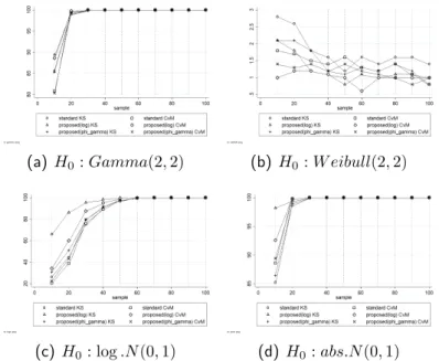
Though both tests are versatile in most settings, but when the support of the data is strictly smaller than the entire real line (let say the support is an interval Ω ⊂ R), the naive kernel distribution function estimator also suffers the boundary problem, as in the naive kernel density estimator. Even though in some cases (e.g. fX(0) = 0 when 0 is the boundary point) the boundary effects of F^b_X(x) is not as severe as in the kernel density estimator, but the problem still occurs. It is because the value of F^b_X(x) is still larger than 0 (or less than 1) at the boundary points. This phenomena cause large value of |F^b_X(x)−F(x)| in the boundary regions, and then KS^d and CvM[ tend to be larger than they are supposed to be, leading to the rejection ofH₀ even though H₀ is right. To make things worse, chapter 4 will illustrate how this problem enlarges type-2 error by accepting the null hypothesis when it is wrong.

1.4 The mean residual life function

Statistical inference for remaining lifetimes would be intuitively more appeal- ing than the popular hazard rate function, since its interpretation as “the risk of immediate failure” can be difficult to grasp. A function called the mean residual life (or mean excess loss) which represents “the average remaining time before failure” is easier to understand. The mean residual life (or MRL for short) function is of interest in many fields relating to time and finance, such as biomedical theory, survival analysis, and actuarial science.

Let us work under the same settings as in section 1.3, where the distribution is supported on an interval Ω ⊂ R, where inf Ω = ω⁰, sup Ω = ω⁰⁰, and

−∞ ≤ ω⁰ < ω⁰⁰ ≤ ∞. Also, let S_X(t) = Pr(X > t) be the survival function, S^X(t) = ^R_t^∞S_X(x)dx be the cumulative survival function, and define a new notation ¯SX(t) =^R_t^∞SX(x)dx. Then

m_X(t) =E(X−t|X > t), t∈Ω (1.20)

(12)

is the definition of the mean residual life function, or can be written as m_X(t) = S^X(t)

S_X(t). (1.21)

For a detailed discussion about the MRL function, see Embrechts et al.

(1997) or Guess and Proschan (1988). Murari and Sujit (1995) and Belzunce et al. (1996) discussed the use of the MRL function for ordering and clas- sifying distributions. On the other hand, Cox (1962), Kotz and Shanbhag (1980), and Zoroa et al. (1990) proposed how to determine distribution via an inversion formula of m_X(t). Ruiz and Navarro (1994) have considered the problem of characterization of the distribution function through the rela- tionship between the MRL function and the hazard rate function. The MRL functions of finite mixtures and order statistics have been studied as well by Navarro and Hernandez (2008).

Some properties and applications of the MRL concept related to oper- ational research and reliability theory in engineering are interesting topics.

While Nanda et al. (2010) discussed the properties of associated orderings in the MRL function, Huynhet al. (2014) studied the usefulness of the MRL models for maintenance decision-making. Another examples are the utiliza- tion of the MRL functions of parallel system by Sadegh (2008), the MRL for records by Raqab and Asadi (2008), the MRL of a k-out-of-n:G system by Eryilmaz (2012), the MRL of a (n −k + 1)-out-of-n system by Poursaeed (2010), the MRL in reliability shock models by Eryilmaz (2017), the MRL subjected to Marshall-Olkin type shocks by Bayramoglu and Ozkut (2016), the MRL of coherent systems by Eryilmaz et al. (2018) and Kavlak (2017), the MRL for degrading systems by Zhao et al. (2018), and the MRL of rail wagon bearings by Ghasemi and Hodkiewicz (2012).

The natural estimator of the MRL function is the empirical one, which is m_n(t) = Sn(t)

Sn(t) =

Pn

i=1(X_i−t)I(X_i > t)

Pn

i=1I(X_i > t) , t ∈Ω, (1.22) where I(A) is the usual indicator function on set A. Yang (1978), Ebrahimi (1991), and Csörgő and Zitikis (1996) studied the properties of m_n(t). Even though it has several good attributes (e.g. unbiasedness and consistency), the empirical MRL function is just a rough estimate of m_X(t) and lack of smoothness. Estimating is also impossible for large t because S_n(t) = 0 for t > max{x₁, x₂, ..., x_n}. Though we can just define m_n(t) = 0 for such case, it is a major disadvantage as analysing the behaviour of the MRL function when t→ ∞ is of an interest.

Various parametric models of MRL have been discussed in literatures, for example the transformed parametric MRL models by Sun and Zhang (2009),

(13)

the upside-down bathtub-shaped MRL model by Shen et al. (2009), the MRL order of convolutions of heterogeneous exponential random variables by Zhao and Balakrishnan (2009), the proportional MRL model by Nandaet al. (2006) and Chanet al. (2012), and the MRL models with time-dependent coefficients by Sun et al. (2012).

Some nonparametric estimators ofm_X(t) which are related to the empirical one have been discussed in a fair amount of literature. For example, Ruiz and Guillamón (1996) estimated the numerator inm_n(t) by a recursive kernel estimate and left the empirical survival function unchanged, while Chaubey and Sen (1999) used the Hille’s Theorem in Hille (1948) to smooth both the numerator and denominator in m_n(t).

The other maneuver that can be used for estimating the MRL function nonparametrically is the kernel method. We need two other functions derived from the kernel K(x), which are

V(x) =

Z ∞ x

K(z)dz and V(x) =

Z ∞ x

V(z)dz. (1.23) Hence, the naive kernel MRL function estimator can be defined as

cm_X(t) = S^bX(t)

Sb_X(t) = h^Pⁿ_i=1V

_t−X

i

h

Pn

i=1V ^t−X_h ⁱ , t∈Ω. (1.24) Guillamón et al. (1998) discussed the asymptotic properties of the naive kernel MRL function estimator in detail.

However, as usuallymX(t) is used for time or finance related data, which are on nonnegative real line or bounded interval, the naive kernel MRL function estimator suffers the boundary bias problem as well. In the case of fX(ω⁰) = 0 (or fX(ω⁰⁰) = 0), the boundary effects of _cmX(t) whent →ω⁰ (or t → ω⁰⁰) is not as bad as in the kernel density estimator, but the problems still occur. It is because the termS_X(ω⁰) and 1−S_X(ω⁰⁰) in theBias[S^bX(ω⁰)]

and Bias[S^b^X(ω⁰⁰)] can never be 0 since SX(ω⁰) = 1−SX(ω⁰⁰) = 1, which meansS^bX(t) causes the boundary problems for_cm_X(t). Moreover, in the case of f_X(ω⁰) > 0 and f_X(ω⁰⁰) > 0 (e.g. uniform distribution), not only S^bX(t), but S^bX(t) also adds its share to the boundary problems for _cmX(t).

To make things worse, the naive kernel MRL function estimator does not preserve one of the most important properties of the MRL function, which is mX(ω⁰) +ω⁰ = E(X). It is reasonable if we expect m_cX(ω⁰) +ω⁰ ≈ X.¯ However, S^b_X(ω⁰) is less than 1 and S^bX(ω⁰) is smaller than the average value ofX_i⁰s, due to the weight that they still put on the outside of Ω. Accordingly, there is no guarantee of how far or how close _cmX(ω⁰) +ω⁰ is to ¯X.

(14)

Though Abdous and Berred (2005) successfully adopted the idea of local linear fitting for the MRL function estimation, in this thesis we are going to try bijective transformation idea to remove the boundary effects. In this situation there are no boundary effects at all, as we will not put any weight outside the support.

(15)

Chapter 2 New Type of Gamma Kernel Density Estimator

In this chapter, we will start our discussion with the formulation of the modified gamma kernel in detail. First we try to use another parameters in gamma density function and then derive its properties. Then, we modify it using some expansions, and calculate further about its new asymptotic properties. At last, we will show the simulation result and compare three kinds of kernel density estimator.

2.1 New type of gamma kernel density estimator formulation

Before starting our discussion, we need to impose assumptions; they are:

A1. The bandwidthh >0 satisfies h→0 and nh→ ∞ when n → ∞, A2. The densityf_X is three times continuously differentiable, and the fourth

derivative f_X⁽⁴⁾ exists,

A3. The following integrals ^R ^h^f_f^X⁰ ^(x)

X(x)

i2

dx, ^Rx⁴^h^f_f^X⁰⁰^(x)

X(x)

i2

dx, ^R x²[f_X⁰⁰(x)]²dx, and ^R x⁶[f_X⁰⁰⁰(x)]²dx are finite.

The first assumption is the usual assumption for the standard kernel density estimator. Since we will use exponential and logarithmic expansions, we need A2 to ensure the validity of our proofs. The last assumption is necessary to make sure we can calculate the MISE.

As we stated before, the modification of the gamma kernel is started by replacing the shape and the scale parameters of the gamma density with

(16)

suitable functions of x and h, and this kernel is defined as a new gamma kernel. Our purpose in doing this is to reduce the variance so that it is smaller than the variance of Chen’s method. After trying several combinations of functions, we chose the density of Gamma(h^−1/2, x√

h+h), which is K(y;x, h) = y^√¹^h⁻¹e⁻

y x

√ h+h

Γ^√¹

h

(x√

h+h)^√¹^h

, (2.1)

as a kernel, and we define the new gamma kernel density “estimator” as A_h(x) =

Pn i=1X

√1 h−1

i e⁻^x^√^Xi^h+h nΓ^√¹

h

(x√

h+h)^√¹^h

, (2.2)

where n is the sample size, and h is the bandwidth.

Remark 2.1.1. Even though the formula in Equation (2.2) can work as a den- sity estimator properly, it is not our proposed method (that is why we put quotation marks around the word “estimator”). As we will state later, we need another modification for Equation(2.2)before our proposed estimator is created.

After this, we need to derive the bias and the variance formulas ofA_h(x).

Consult the following theorem.

Theorem 2.1.2. Assuming A1 and A2, for the functionA_h(x)in Equation(2.2), its bias and variance are

Bias[A_h(x)] =

f_X⁰ (x) + 1

2x²f_X⁰⁰(x)

√

h+o(√

h) (2.3)

and

V ar[A_h(x)] =











R²

√1 h−1

fX(x) 2(x+√

h)

√

π(1−√ h)R

√2 h−2

nh¹⁴

+O

h¹⁴ n

, ^x_h → ∞

R²

√1 h−1

fX(x) 2(c√

h+1)

√

π(1−√ h)R

√2 h−2

nh³⁴

+O

1 nh¹⁴

, ^x_h →c,

(2.4)

for some positive number c and

R(z) =

√2πz^z+¹²

e^zΓ(z+ 1). (2.5)

(17)

Remark 2.1.3. The function R(z) (Brown and Chen 1999) monotonically in- creases with limz→∞R(z) = 1 and R(z)<1, which means ^R

2(_h¹⁻¹)

R(h²−2) ≤1. From these facts, we can conclude that V ar[A_h(x)] is O(n⁻¹h^−1/4) when x is in the interior, and it isO(n⁻¹h^−3/4)when xis near the boundary. Both of these rates of convergence are faster than the rates of the variance of Chen’s gamma kernel estimator for both cases, respectively. Furthermore, instead ofx^−1/2,V ar[A_h(x)]

depends on (x+√

h)⁻¹, which means the value of the variance will not speed up to infinity when x approaches 0.

Even though we have succeeded in reducing the order of the variance, we now encounter a larger bias order. To avoid this problem, we use geometric extrapolation to change the order of bias back to h.

Theorem 2.1.4. Let A_h(x) be the function in Equation (2.2). Assuming A1 and A2, if we define J_h(x) =E[A_h(x)], then

[J_h(x)]²[J_4h(x)]⁻¹ =f_X(x) +O(h). (2.6) Remark 2.1.5. The functionJ_4h(x)is the expectation of the function in Equa- tion (2.2) with 4h as the bandwidth. Furthermore, the term after f_X(x) in Equation(2.6)is in the orderh, which is the same as the order of bias for Chen’s gamma kernel density estimator. This theorem will lead us to the idea to modify A_h(x). We present the explicit asymptotic formula of O(h) in the appendices.

Theorem 2.1.4 gives us the idea to modify A_h(x) and to define our new estimator. Hence, we propose

feX(x) = [Ah(x)]²[A4h(x)]⁻¹ (2.7) as the modified gamma kernel density estimator, our proposed method. This idea is actually straightforward. It uses the fact that the expectation of the operation of two statistics is asymptotically equal (in probability) to the operation of the expectation of each statistic. Though we do not use any concept of convergence in probability in our proofs, the idea is still applicable when using Taylor Expansion.

For the bias of our proposed estimator, we have the following theorem.

Theorem 2.1.6. Assuming A1 and A2, the bias of the modified gamma kernel density estimator is

Bias[f^e_X(x)] =−2

"

b(x)− a(x) 2fX(x)

#

h+o(h) +O

1 nh¹⁴

, (2.8)

(18)

where

a(x) =f_X⁰ (x) + 1

2x²f_X⁰⁰(x) (2.9)

b(x) =

x+ 1 2

f_X⁰⁰(x) +x²

x 3 +1

2

f_X⁰⁰⁰(x). (2.10) As expected, the bias’ leading term is actually the same as the explicit form of O(h) in theorem 2.1.4 (see appendices). Its order of convergence changed back toh, the same as the bias of Chen’s method. This is quite the accomplishment because if we can keep the order of the variance the same as V ar[A_h(x)], we can then conclude that the MSE of our modified gamma kernel density estimator is smaller than the MSE of Chen’s gamma kernel estimator. However, before jumping into the calculation of variance, we need the following theorem.

Theorem 2.1.7. Assuming A1 and A2, for the function in Equation (2.2) with bandwidth h,A_h(x), and with bandwidth 4h, A_4h(x), the covariance of them is equal to

Cov[Ah(x), A4h(x)] = R^√¹

h −1R ¹

2√ h −1 2√

πR ³

2√

h −2(3x+ 5√ h)

₃

2 −2√ h

3 2

√ h−³

2

(2−2√

h)^√¹^h⁻¹²(1−2√

h)²^√¹^h⁻¹²

× x+√ h 3x+ 5√ h

! ¹

2

√ h−1

2x+ 4√ h 3x+ 5√

h

!^√¹

h−1

f_X(x) nh¹⁴ +O





h¹⁴ n



, when xh⁻¹ → ∞, and

Cov[A_h(x), A_4h(x)] = R^√¹

h −1R ¹

2√ h −1 2√

πR ³

2√

h −2(3c√ h+ 5)

3 2 −2√

h

3 2√

h−³

2

(2−2√

h)^√¹^h⁻¹²(1−2√

h)²^√¹^h⁻¹²

× c√ h+ 1 3c√

h+ 5

!₂^√¹_h⁻¹

2c√ h+ 4 3c√

h+ 5

!^√¹_h⁻¹

f_X(x) nh³⁴ +O

1 nh¹⁴

, when xh⁻¹ →c >0.

Theorem 2.1.8. Assuming A1 and A2, the variance of the modified gamma kernel density estimator is

V ar[f^e_X(x)] = 4V ar[A_h(x)] +V ar[A_4h(x)]−4Cov[A_h(x), A_4h(x)] +o

1 nh¹⁴

, where its orders of convergence areO(n⁻¹h^−1/4)in the interior andO(n⁻¹h^−3/4) in the boundary region.

(19)

As a conclusion to theorems 2.1.6 and 2.1.8, with the identity of MSE, we have

M SE[f^e_X(x)] =











O(h²) +O

1 nh¹⁴

, ^x_h → ∞ O(h²) +O

1 nh³⁴

, ^x_h →c.

(2.11)

The theoretical optimum bandwidths are h = O(n^−4/9) in the interior and O(n^−4/11) in the boundary region. As a result, the optimum orders of convergence are O(n^−8/9) andO(n^−8/11), respectively. Both of them are smaller than the optimum orders of Chen’s estimator, which are O(n^−4/5) in the interior and O(n^−2/3) in the boundary region. Furthermore, since the MISE is just the integration of MSE, it is clear that the orders of convergence of the MISE are the same as of the MSE.

Calculating the explicit formula of M ISE(fê_X) is nearly impossible because of the complexity of the formulas ofBias[fê_X(x)] andV ar[fê_X(x)]. How- ever, there is one thing we would like to discuss regarding this matter. Us- ing a similar argument stated by Chen (2000), the boundary region part of V ar[fê_X(x)] is negligible while integrating the variance. Thus, instead of computing ^R_boundaryV ar[fê_X(x)] +^R_interiorV ar[fê_X(x)], it is sufficient to just calculate ^R₀^∞V ar[fêX(x)]dx using the formula of the variance in the interior.

With that, computing M ISE(f^e_X) =

Z ∞ 0

Bias²[f^e_X(x)]dx+

Z ∞ 0

V ar[f^e_X(x)]dx

can be approximated by using numerical methods (assuming f_X is known).

2.2 Simulation studies

In this section, we provide the results of a simulation study we did to show the performances of our proposed method and compare them with other estimators’ results. The measures of error we use in this thesis are the MISE, the MSE, bias, and variance. Since we are working under assumptions A1, A2, and A3, the MISE of our proposed estimator is finite. We calculated the average integrated squared error (AISE), the average squared error (ASE), simulated bias, and simulated variance, with a sample size of n = 50 and 10000 repetitions for each case.

We compared four gamma kernel density estimators: Chen’s gamma kernel density estimator f^b_C(x), two nonnegative bias-reduced Chen’s gamma estimatorsf^b_KI1(x) andf^b_KI2(x) (Igarashi and Kakizawa 2015, eq. 10 and 11),

(20)

and our modified gamma kernel density estimator f^e_X(x). We generated several distributions for this study; they are exponential distribution exp(1/2), gamma distribution Gamma(2,3), log-normal distribution log.N(0,1), in- verse Gaussian distributionIG(1,2), Weibull distributionW eibull(3,2), and absolute normal distribution abs.N(0,1). The least squares cross-validation technique was used to determine the value of the bandwidths.

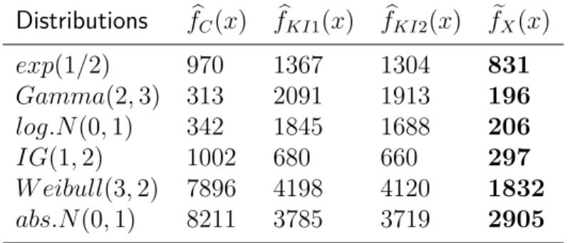
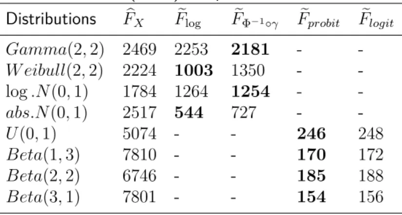
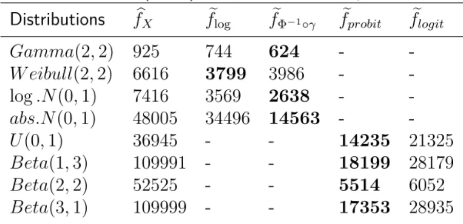
Table 2.1 compares AISEs, representing the general measure of error. As we can see, the proposed method outperformed the other estimators. Since one of our main concerns is eliminating the boundary bias problem, it is necessary to take our attention to the values of the measures of error in the boundary region. Tables 2.2, 2.3, and 2.4 show the ASE, bias, and variance of those four estimators whenx= 0.01. Once again, our estimator had the best results. Though the differences among the values of bias were relatively not big (Table 2.3), from Table 2.4, we can witness how our variance reduction has an effect.

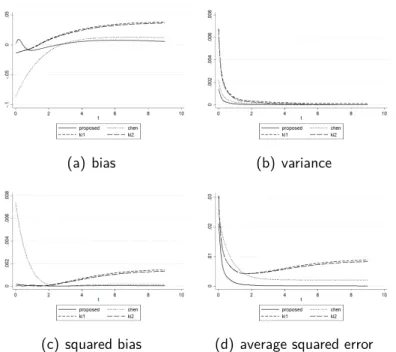
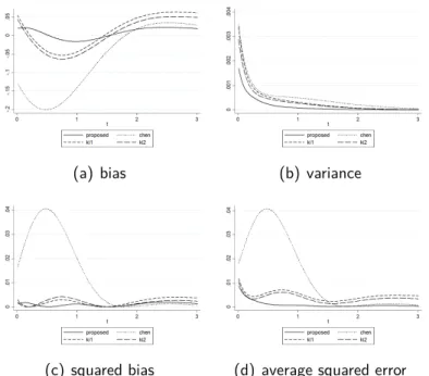
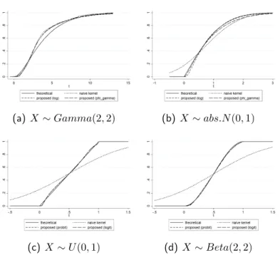
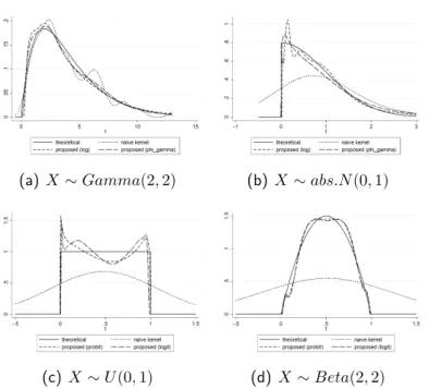
As further illustrations, we also provide graphs of point-wise ASE, bias, squared bias, and variance to compare our estimator’s performances with those of the others. We generated exponential, gamma, and absolute normal distributions 1000 times to produce Figs. 2.1, 2.2, and 2.3.

In some cases, we found that the bias value of our proposed estimator was away from 0 more than the other estimators (e.g., Fig. 2.1(a) around x = 1, Fig. 2.2(a) around x= 4, and Fig. 2.3(a) around x = 0.2). Though this could reflect poorly on the proposed estimator, from the variance parts (Figs. 2.1(b), 2.2(b), and 2.3(b)), we see that our estimator never failed to give the smallest value of variance, confirming that we succeeded in reducing variance with our method. Moreover, the result of the variance reduction is the reduction of point-wise ASE itself, shown in Figs. 2.1(d), 2.2(d), and 2.3(d). One may take note of Fig. 2.2(d) when x ∈ [1,4] because the estimators of Igarashi and Kakizawa slightly outperformed the proposed method. However, as x got larger, ASE[f^b_KI1(x)] and ASE[f^b_KI2(x)] failed to get closer to 0 (they will when x is large enough), while ASE[f^e_X(x)]

approached 0 immediately.

(21)

Table 2.1: Comparison of the average integrated squared error (×10⁵) Distributions f^bC(x) f^bKI1(x) f^bKI2(x) f^eX(x)

exp(1/2) 970 1367 1304 831 Gamma(2,3) 313 2091 1913 196 log.N(0,1) 342 1845 1688 206

IG(1,2) 1002 680 660 297

W eibull(3,2) 7896 4198 4120 1832 abs.N(0,1) 8211 3785 3719 2905

Table 2.2: Comparison of the average squared error (×10⁵) when x= 0.01 Distributions f^bC(x) f^bKI1(x) f^bKI2(x) f^eX(x)

exp(1/2) 1600 1547 1553 991 Gamma(2,3) 207 384 359 168 log.N(0,1) 36 178 160 34

IG(1,2) 1006 829 781 422

W eibull(3,2) 1528 708 643 304 abs.N(0,1) 2389 2018 1999 721 Table 2.3: Comparison of the bias (×10⁴) when x= 0.01

Distributions f^b_C(x) f^b_KI1(x) f^b_KI2(x) f^e_X(x) exp(1/2) −1054 −1865 −1904 −858 Gamma(2,3) 391 583 561 233 log.N(0,1) 150 417 395 120

IG(1,2) 961 869 840 386

W eibull(3,2) 1215 821 780 342 abs.N(0,1) −1383 303 297 157 Table 2.4: Comparison of the variance (×10⁵) when x= 0.01

Distributions f^b_C(x) f^b_KI1(x) f^b_KI2(x) f^e_X(x) exp(1/2) 490 1465 1469 244

Gamma(2,3) 54 43 44 11

log.N(0,1) 39 36 36 35

IG(1,2) 835 739 753 273

W eibull(3,2) 532 340 343 184 abs.N(0,1) 476 1926 1910 211

(22)

(a) bias (b) variance

(c) squared bias (d) average squared error

Figure 2.1: Comparison of point-wise bias, variance, and ASE of f^e_X(x), f^b_C(x), fb_KI1(x), and f^b_KI2(x) for estimating density of exp(1/2)with sample size 150.

Figure 2.2: Comparison of the point-wise bias, variance, and ASE of f^e_X(x), fb_C(x),f^b_KI1(x), andf^b_KI2(x)for estimating density ofGamma(2,3)with sample size 150.

(23)

Figure 2.3: Comparison of the point-wise bias, variance, and ASE of f^e_X(x), fb_C(x), f^b_KI1(x), and f^b_KI2(x) for estimating density of abs.N(0,1) with sample size 150.

(24)

Chapter 3 Modified Kernel Distribution Function Estimator

We will start our discussion in this chapter with the derivation of our proposed distribution function estimator. After that, we present our calculation for the bias and the variance to show our estimator is theoretically better than the standard one. At last, we will show the simulation study.

3.1 MISE reduction by geometric extrapolation

In this section, we will apply geometric extrapolation method to the kernel distribution function estimator, in order to reduce bias. The idea of reducing bias by geometric extrapolation is doing a self-elimination technique between two standard kernel distribution function estimators with different bandwidths, with some helps of exponential and logarithmic expansions. By doing that, vanishing the h² term of the asymptotic bias is possible, and the the order of convergence changes to h⁴.

Before starting our main purpose, we need to impose some assumptions, they are:

B1. The kernel K is a nonnegative continuous function, symmetric about 0, and it integrates to 1,

B2. The integral^R_−∞^∞ w⁴K(x)dw is finite,

B3. The bandwidthh >0 satisfies h→0 and nh→ ∞ when n → ∞, B4. The densityf_X is three times continuously differentiable, and the fourth

derivative f_X⁽⁴⁾ exists,

(25)

B5. The integrals^R_−∞^∞ ^[f_F^X⁰ ^(x)]²

X(x) dx and ^R_−∞^∞ f_X⁰⁰⁰(x)dx are finite.

The first and third ones are the usual assumptions for the standard kernel distribution function estimator. Since we will use exponential and logarithmic expansions, we need B2 and B4 to ensure the validity of our proofs. For the last assumption, it is necessary to make sure we can calculate MISE.

We now ready to begin the explanation about how to modify the standard kernel distribution function estimator and reduce its bias. First, we have this following theorem.

Theorem 3.1.1. Letj_h(x) =E[F^b_h(x)]anda(6= 1)be a positive number. Under the assumptions B1-B4, we have

[j_h(x)]^t¹[j_ah(x)]^t² =F_X(x) +O(h⁴), (3.1) where t₁ = _a₂^a₋₁² and t₂ =−_a₂¹₋₁.

Remark 3.1.2. The function j_ah(x) is an expectation of the standard kernel distribution function estimator with ah as the bandwidth, that is, j_ah(x) = E[F^b_ah(x)], where

Fb_ah(x) = 1 n

n

X

i=1

W

x−X_i ah

.

Furthermore, the term afterF_X(x)in (3.1) is in the order ofh⁴, which is smaller than the order of bias of the standard kernel distribution function estimator. Even though this theorem does not state about a bias of some estimator, it will lead us to the idea to modify the standard kernel distribution function estimator. About the explicit asymptotic formula of O(h⁴), we will present it in the appendices.

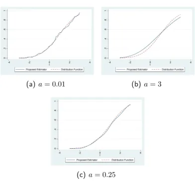
The theorem 3.1.1 gives us an idea to modify kernel distribution function estimator which will have, intuitively, similar property for bias. Hence, we propose a new estimator of distribution function as

FeX(x) = [F^bh(x)]

a2

a2−1[F^bah(x)]⁻â²¹⁻¹. (3.2) Remark 3.1.3. As we can see, the number a acts as the second smoothing parameter here, because it controls the smoothness of F^b_ah (since it is placed inside the function W) and determines how much the effect of F^b_h and F^b_ah as a part of their power. Larger a means the effect of F^b_h is larger for Fê_X, and vice versa. Furthermore, whena → ∞, we will find thatFê_X →F^b_h. Oppositely, when a really close to 0, the effect of F^b_h is almost vanished. However, different with bandwidth h, the number a is purely our choice and does not depend on the sample sizen. Lettingatoo close to0is not wise, since it acts as a denominator in the argument of function W.