INVITED PAPER Special Section on Smart Radio and Its Applications in Conjunction with Main Topics of SmartCom
Orbital Angular Momentum (OAM) Multiplexing: An Enabler of a New Era of Wireless Communications
Doohwan LEE†a), Hirofumi SASAKI†, Hiroyuki FUKUMOTO†, Ken HIRAGA†,Members, andTadao NAKAGAWA†,Senior Member
SUMMARY This paper explores the potential of orbital angular mo- mentum (OAM) multiplexing as a means to enable high-speed wireless transmission. OAM is a physical property of electro-magnetic waves that are characterized by a helical phase front in the propagation direction.
Since the characteristic can be used to create multiple orthogonal channels, wireless transmission using OAM can enhance the wireless transmission rate. Comparisons with other wireless transmission technologies clarify that OAM multiplexing is particularly promising for point-to-point wireless transmission. We also clarify three major issues in OAM multiplexing:
beam divergence, mode-dependent performance degradation, and reception (Rx) signal-to-noise-ratio (SNR) reduction. To mitigate mode-dependent performance degradation we first present a simple but practical Rx antenna design method. Exploiting the fact that there are specific location sets with phase differences of 90 or 180 degrees, the method allows each OAM mode to be received at its high SNR region. We also introduce two methods to address the Rx SNR reduction issue by exploiting the property of a Gaus- sian beam generated by multiple uniform circular arrays and by using a dielectric lens antenna. We confirm the feasibility of OAM multiplexing in a proof of concept experiment at 5.2 GHz. The effectiveness of the pro- posed Rx antenna design method is validated by computer simulations that use experimentally measured values. The two new Rx SNR enhancement methods are validated by computer simulations using wireless transmission at 60 GHz.
key words: orbital angular momentum multiplexing, uniform circular array, Gaussian beam, Bessel beam, lens antenna
1. Introduction
Recent decades have witnessed significant progress in wire- less communication technologies. In particular, the utiliza- tion of higher frequency bands (e.g., millimeter-wave (mm- wave) band), where bandwidth of several GHz is available, has played a key role in achieving such progress[1],[2].
Recent explosive research efforts have shown the feasibility and possibility of utilizing mm-wave technologies to provide up to several tens of Gbps transmission[3].
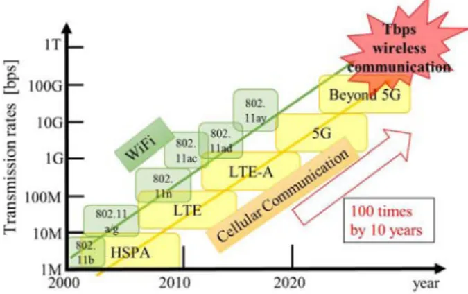
Despite such achievements, providing high-order data- rate transmission is expected to be necessary to satisfy the ever increasing demand for such transmission for the next coming decade. From reading the history we have also observed the transmission rate of wireless communication has increased 100 folds every 10 years as shown in Fig. 1.
Considering this trend and the current mature status of mm- wave technologies[4], we consider it is time to discuss what
Manuscript received September 5, 2016.
Manuscript revised November 30, 2016.
Manuscript publicized January 12, 2017.
†The authors are with NTT Network Innovation Laboratories, NTT Corporation, Yokosuka-shi, 239-0847 Japan.
a) E-mail: [email protected].
DOI: 10.1587/transcom.2016SCI0001
Fig. 1 Evolution trend of wireless communication technologies and transmission rates.
will be candidates of wireless transmission technologies to provide up to 1 Tbps transmission.
It is expected that the provision of such higher-rate transmission is needed for wireless fronthaul and/or back- haul since extremely large volume of wireless data traffic will be transferred. Here, wireless fronthaul refers to wire- less links between remote radio heads and central baseband units, and wireless backhaul refers to wireless links between base stations and the core network [5]. When the usage of the mm-wave band is taken into account, distances be- tween transmitter (Tx) and receiver (Rx) antennas of such wireless fronthaul and/or backhaul are generally considered from several tens of meters to 100 meters. Since these wire- less fronthaul and/or backhaul are typically expected to be point-to-point wireless links, we focus our discussion on the point-to-point wireless transmission.
In this paper, we first explore four promising candi- date technologies: massive MIMO (multiple-input multiple- output) [6]–[8], short-range MIMO [9]–[11], line-of-site (LOS) MIMO [12]–[14], and orbital angular momentum (OAM) multiplexing [15]–[17]. Then, while not denying the possibilities of other technologies, we put the main con- cern on OAM multiplexing since currently it seems the most promising way to achieve higher rates for point-to-point wire- less transmission with reasonable circuit complexity.
The OAM multiplexing method is an emerging wireless transmission technology that exploits a physical property of electro-magnetic waves characterized by a helical phase front in the propagation direction [15]. The propagating beams with a distinct number of phase rotations, i.e., OAM Copyright©2017 The Institute of Electronics, Information and Communication Engineers
modes, are orthogonal to one another and create multiple orthogonal channels. This technology is also in a similar vein with the MIMO technologies in that it uses multiple antenna elements. The elements are used to generate superposition of multiple beams carrying different OAM modes.
From the wireless communication perspective, the beauty of OAM multiplexing is that it generates multiple orthogonal channels in a LOS channel environment without complex signal processing such as channel diagonalization.
If one considers the growing importance of LOS chan- nel environments in mm-wave and/or higher frequency bands [18], [19], this advantage of OAM multiplexing deserves further exploitation to achieve the desired higher-rate trans- mission. This paper mainly considers a LOS channel envi- ronments where non-dominant paths are negligible. There were many measurement results that experimentally mea- sured path loss models were almost close to the free-space path loss model so that non-dominant components can be negligible[19, and the references therein]. Cases where the effect of non-dominant paths is non-trivial are additionally discussed with respect to the tradeoffs between complexity and performance in Sect. 9.
To explore these possibilities, we investigated the per- formance of wireless communications using OAM multi- plexing in terms of capacity, multiplexing and demultiplex- ing, channel coding, interleaving, modulation level, and power control. We also clarified the most significant chal- lenges that hinder the potential of OAM multiplexing. They are beam divergence, reception signal-to-noise-ratio (SNR) degradation, and mode dependency of the performance. The higher the OAM mode, the more severe the beam divergence becomes. This results in the need for larger Rx antennas or reduced Rx SNR.
To address these issues we provide a practical and novel Rx antenna design and corresponding signal separa- tion methods. We also present two Rx SNR enhancement methods using a dielectric lens and multiple uniform circular arrays (UCAs). The feasibility of the Rx antenna design is validated by proof of concept experiments and simulations using those experimental results. Also, the effectiveness of the Rx SNR enhancement methods is shown by a simulation study.
The rest of the paper is organized as follows: Section 2 describes related work regarding other candidate wireless transmission technologies and OAM multiplexing. Section 3 provides background of the OAM multiplexing and summa- rizes its challenges. Section 4 describes the proposed an- tenna design and Sect. 5 explains the Rx SNR enhancement methods to address the challenges. The evaluation results obtained by proof of concept experiments and related sim- ulations are given in Sect. 6. Extended evaluations results obtained by simulations are given in Secs. 7 and 8. We pro- vide addition discussion in Sect. 9 and conclude the paper with a summary in Sect. 10.
2. Related Work
In this section we will first describe candidate technologies to enable higher rate wireless transmission: massive MIMO [6]–[8], short-range MIMO[9]–[11], and LOS MIMO[12]–
[14] technologies. Then, we will describe the history of OAM multiplexing technology and review the published lit- erature for it.
2.1 Related Wireless Transmission Technologies
Massive MIMO is a technology that utilizes multiple an- tennas in collaboration with beam-forming technology to increase the capacity. It enables both high transmission distance and transmission rate when used for mm-wave fre- quency band transmission. Many simulation studies and field experiments have been successfully conducted, and standardization work has been also done in parallel [20].
Massive MIMO basically aims to provide a higher rate trans- mission to multiple users by proper beam-forming[6]–[8].
Therefore, it is a suitable way to enhance the total transmis- sion rate for point to multi-point wireless transmission such as downlink transmissions in cellular communications.
Short-range MIMO is a special type of MIMO technol- ogy for usage over short-range distances (within several ten centimeters) where the propagation environment is typically specified by the LOS channel [9]–[11]. To provide con- current multiple-stream transmission under a LOS channel, distances among antenna elements are properly customized to get low spatial correlations[9]. Recent work and stan- dardization approaches are aiming to achieve transmission rate up to 100 Gbps by transmitting 16 concurrent streams [21]. If one takes the continuous efforts that have been re- ported in the literature into account, it can be considered that higher-rates than currently exist could be feasible, as long as the usage is limited to a short-rage distance.
LOS MIMO is also a special type of MIMO technology that makes it possible to increase the number of concurrent transmissions under LOS channel environments[12]–[14].
Positions of antenna elements are properly tuned to make Euclidian distance differences from Tx antennas at an Rx antenna to be odd multiples of half-wavelength. Elaborately combined with 90- and 180-degree phase shifters, interfer- ences from other streams are cancelled out. Like OAM mul- tiplexing, this technology allows multiple concurrent trans- missions even in a LOS channel environment. However, the cases are typically limited by2×2or4×4due to the specific conditions of the phase differences[22]. Also, the fact that the optimum antenna configuration varies with the distance between Tx and Rx hinders the flexibility of the deployment where a wide variety of distances between Tx and Rx is supposed to be allowed.
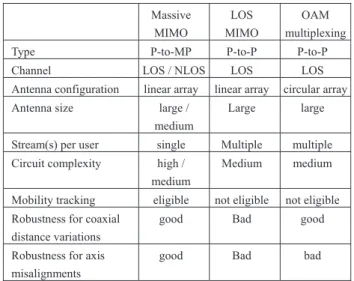
Table 1 provides comparison of these technologies in various aspects when they are used in the mm-wave band for a fixed wireless link of which distance is from around several of tens meters to 100 meters. Short-range MIMO is not
Table 1 Comparison of massive MIMO, LOS MIMO, and OAM multi- plexing for fixed wireless links such as wireless fronthaul and/or backhaul using mm-wave band (P-to-P, P-to-MP, LOS, and NLOS are respectively point-to-point, point-to-multi point, line-of-sight, and non-line-of-sight).
included in this table because it is the specialized case of LOS MIMO of which distance is less than several tens centimeters.
Note that this is overall trend and some variations might exist. For example, although massive is classified as a P-to- MP (point-to-multi point) technology that supports a single stream per user in Table 1, it is also possible to support P-to-P (point-to-point) system by applying precoding that enables multi-stream transmission. Note also that the circuit complexity of massive MIMO[23]is estimated higher than those of LOS MIMO and OAM multiplexing considering the support for the usage in the NLOS channel environments and usage of the mobility tracking.
To provide multiple concurrent streams’ point-to-point wireless communication in a LOS channel environment while considering the practical versatility of the deployment, we gave highest scores to OAM multiplexing and proceeded to carry out further studies.
2.2 Related Work in OAM multiplexing
Study on electro-magnetic waves carrying OAM modes has a long history. Some work in this field dates from the early 1900s[24]. In the 1980s, the multiplexing concept using OAM modes had been already suggested by circular array antenna researchers[25]. From the late 1990s to the 2000s similar concepts were studied in various fields including radio astronomy[26], photonics [27],[28], and free-space wireless communication [29], [30]. Exploitation of OAM carrying beams for the wireless communication using very- high frequency (VHF) or ultra-high frequency (UHF) band has been beyond practical feasibility due to the physical size of antenna. From the early 2010s interest was drawn again to the wireless communication field, influenced by matur- ing technologies using mm-wave band communications that enable the physical antenna size to be small.
After interesting and fruitful debates whether OAM
multiplexing was a purely new technology or not[31]–[33], it has come to be regarded as a subset of MIMO technology by the majority of researchers in the wireless communica- tion field as long as the OAM beams are generated by the array antennas. However, OAM multiplexing is attractive as a way to provide higher-rate transmission in an LOS channel environment without the need for complex signal processing such as channel diagonalization.
Studies regarding OAM multiplexing in the wireless communication field are categorized into antenna design and beam generation [34]–[38], proof of concept experiments [15], [16], [35], signal processing method [39]–[41], and system study such as capacity analysis and link budget[42]–
[44].
Much work has contributed to the antenna design and beam generation after interest was rebooted in the early 2010s. Various types of antenna designs were reported using helicoidally deformed parabolic antennas[34], spiral phase plates (SPP)[15],[16],[35], holographic plates (HP)[35], elaborately tuned planer SPPs [36], and so on [37],[38].
Despite some reports of successful transmissions, it seems to be hard to perform multiplexing in a practical manner us- ing such antennas since each OAM mode needs a differently located antenna. On the other hand, a UCA and/or multiple UCAs[39]–[41]are considered to be suitable for the multi- plexing because they can transmit coaxially aligned multiple streams simultaneously.
The feasibility of OAM multiplexing has been validated in many different experiments [15],[16],[35]. Yan et al.
successfully demonstrated 32 Gbps OAM multiplexing over a 60 GHz mm-wave band with four concurrent OAM modes (Mode =−3,−1, 1, and 3) with 16 QAM modulation[14].
The transmission distance was 2.5 meters and 4 SPPs are used for multiplexing with a 4-to-1 combiner. Mahmouli et al. conducted 4 Gbps uncompressed video transmission over a 60 GHz mm-wave band using HP and SPP[35]. However, as yet no Gbps level transmission experiments over 10 meters have been reported.
The thorough capacity analysis in[42]revealed the ca- pacity upper limit of OAM multiplexing is not superior to that of MIMO technology as long as a UCA is used for OAM beam generation. Mohammadi et al. investigated a system level performance [43]. The link budget was analyzed in [44]while clarifying the mode dependency of the propaga- tion loss. In addition to the above cited work, many other important studies have been done and are still ongoing, such as studies on calibration methods[45], analysis of the effects of multipaths[46]and so on[47],[48].
3. Background and Challenges
3.1 System Model
Figure 2 shows the block diagram of the system model. Other than OAM multiplexing and demultiplexing blocks, the sys- tem model is almost the same as that for current wireless communication systems.
Fig. 2 Block diagram of wireless communication using OAM multiplex- ing.
The transmitter generates data and conducts typical baseband processing such as modulation, interleaving, chan- nel coding, and/or power pre-compensation. The output stream is divided into multiple streams by serial-to-parallel conversion (S/P block in Fig. 2). Then, each stream is up- converted to an RF signal after the digital-to-analog conver- sion (DAC). Each RF stream generates a beam carrying dif- ferent OAM modes using a UCA or multiple UCAs. Then, all OAM signals are simultaneously transmitted over the same frequency band. Note that the OAM beam generation and multiplexing are done by devices such as phase shifters and combiners that do not need the digital signal processing.
If one considers the usage scenario, almost all previ- ous work in the literature has used the free-space propaga- tion channel model or the AWGN (additive white Gaussian noise) channel model. We also followed those channel mod- els where no multipaths existed. However, some necessary discussion regarding the effect of multipaths is added in Sect. 9. In the considered channel, the amplitude and phase of the received signals are only determined by the distance of antenna elements between Tx and Rx.
The OAM demultiplexing is conducted with the re- ceived signal bearing multiple OAM modes and multiple steams are obtained. All streams are down-converted into the baseband and sampled by analog-to-digital converters (ADCs). Note that DAC and ADC are conducted not per antenna element but per OAM mode to reduce the device volume and power consumption. This approach is a simi- lar to that of analog and/or hybrid beamforming of massive MIMO in mm-wave wireless transmission[49],[50]. Con- sequently, each OAM mode signal is obtained after parallel- to-serial conversion and necessary signal processing such as channel-decoding, de-interleaving, and demodulation.
3.2 Beam Generation and Separation
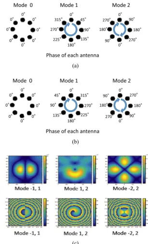
To generate the beam carrying the OAM moden(L =n), antenna elements are connected with phase shifters that make n×360degrees of rotation. Figure 3(a) shows an example of beam generations of OAM mode 0, 1, and 2 using UCAs consisting of 8 antenna elements. Note that it is possible to use either a single UCA or multiple UCAs for multiple OAM mode generation. In the former case, superposed beams are transmitted by a single UCA. In the latter case, concentric
Fig. 3 (a) Generation of OAM modes with a UCA, (b) Separation of OAM modes with a UCA, (c) Intensity distribution (above) and phase distribution (below) of combined OAM modes.
multiple UCAs are used.
The separation of beams carrying OAM modes can be done in a way similar to that for generation using antenna elements connected with phase shifters that make opposite rotation directions. As long as the number of antenna el- ements is larger than 2n, rotations ofn×360 degrees are orthogonal to one another. Therefore, each OAM mode can be separated from mixed OAM modes’ signals without aliasing. Figure 3(b) shows an example of each antenna element phase corresponding to the example above. Such beam separation can also be done by using a single UCA or multiple UCAs as in the beam generation. Note that a divider is equipped between antenna elements and phase shifters in the former case. To avoid confusion regarding the term “multiple UCAs”, hereafter, we will consider only superposition-based beam generation using a single UCA is considered. The usage of the term “multiple UCAs” will be reserved for the Gaussian beam generation described in Sect. 5.
3.3 Properties of OAM Beams
Figure 3(c) shows some examples of intensity and phase distributions of beams carrying multiple OAM modes gen-
erated by a single UCA. At the receiver the diffraction pattern generated by a single transmitting UCA is calculated by the summation of the electric field generated from each antenna element. Since the diffraction pattern of the UCA can be approximated as a Bessel beam[45], the electric field distri- bution of the beam carrying OAM modeLis often expressed by the Bessel beam’s equation as below.
vL(r, θ,z)= λexp[(2πi/λ)√
r2+z2] 4π√
r2+z2 ·i−Lexp[iLθ]·JL
( 2πr D λ√
r2+z2 )
, (1) where JL(·), λ, and D respectively denote the Lth order Bessel function of the first kind, the wavelength of the car- rier frequency, and the radius of the transmitting UCA. Equa- tion (1) is represented in cylindrical coordinates, whererand θare respectively radius and azimuthal angle at the Rx plane that is vertical to the beam propagation direction. zis the distance between the centers of the Tx and Rx UCAs.
Under the free-space propagation or AWGN channel, the intensity and phase of the received signals at a certain location can be analytically obtained by Eq. (1) with param- eters of the radius (D) of the Tx UCA, wavelength (λ), and theLthof the Bessel function of the first kind (JL(·)).
3.4 Challenges
This subsection highlights three major issues that have to be resolved to fully exploit the potential of OAM multiplexing.
These issues are as follows.
•Beam Divergence:
Beams carrying OAM modes diverge along with their prop- agation as shown in Fig. 5. Other than the OAM mode 0, the location of the first Rx peak intensities of OAM modes diverges as propagation distance[51]. It may be considered that various beam forming technologies[52] can generate a sharp non-OAM carrying beam of which divergence is not significant. However, the divergence of OAM carrying beams is determined by the Tx UCA radius and wavelength.
It is therefore necessary to increase the physical size of the Tx UCA or to use higher frequency in order to reduce the divergence of OAM carrying beams. Since both Tx an- tenna size and frequency band are usually not tunable design factors, as of now, we leave this issue as an open problem while suggesting that Tx antenna size be set to be as large as the physical environment allows. Instead, we focus on the following two issues in this paper.
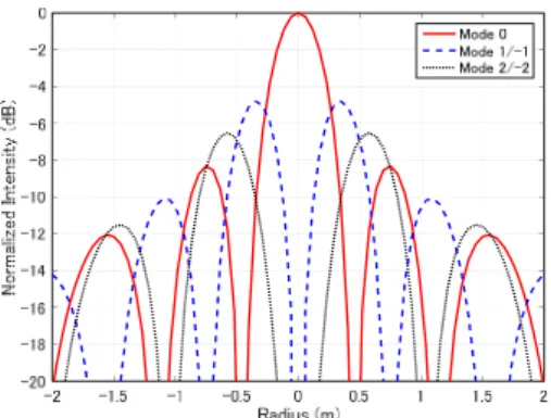
•Rx Power Dissipation by Harmonics of Peak Intensities:
The Rx intensity distributions of an OAM carrying beams generated by a single UCA have many harmonics of peaks as shown in Fig. 4. This dissipates the Rx energy to a wide area, causing not only overall Rx SNR degradation but also inter- ference enhancement to other nearby systems. This issue remains even though larger Tx antenna size or higher fre- quency bands are used as long as OAM beams are generated
Fig. 4 Normalized intensities of the Bessel function of the first kind.
Fig. 5 Conceptual drawing of OAM beam divergence.
by a single UCA. This may eventually limit the transmission distance because the Rx energy is wasted by their harmonics.
•Mode-Dependent Performance Degradation:
The beam carrying different OAM mode yields a different location of the peak intensity. This non-identical peak Rx in- tensity results in mode-dependent performance degradation in accordance with the location of the Rx antenna. Also, the required Rx antenna size to capture the peak Rx power becomes bigger as the number of OAM modes increases as shown in Fig. 4. If the Rx antenna size is limited to a cer- tain size, some OAM modes might not have the peak Rx power. Correspondingly, the performance degradation for higher OAM modes becomes more severe.
These issues are indeed related to one another to some extent. Mainly to deal with the second issue, we present two Rx SNR enhancement methods using multiple UCAs and a dielectric lens in Sect. 5. Mainly to address the third issue, we propose a novel Rx antenna design in Sect. 4. Also the pre-compensation of the transmission power and interleav- ing are applied to average the mode-dependent performance degradation.
4. Proposed Reception Antenna and OAM Beam Sepa- ration
4.1 Reception Antenna Design
If one considers the distinct beam propagation and diver- gence among OAM modes, it may be a good approach to
Fig. 6 Rx antenna proposal.
put the Rx antenna for each OAM mode at its optimum or near-optimum location. For example, the usage of many concentric Rx UCAs that capture OAM modes at their high Rx SNR region may lessen mode-dependent performance degradation. In such concentric Rx UCAs cases, without loss of generality, the outer UCA is used for the reception of a higher OAM mode. Since the UCA antenna radius in- creases by the power of two in such cases, a spacious antenna is necessary to capture the higher OAM mode signals in this approach.
To provide a practical solution that allows higher OAM mode signals to be received at high Rx SNR while main- taining reasonable antenna size, we present a simple but practical reception antenna design and corresponding beam separation method. Our idea uses the fact that there are spe- cific location sets of which phase differences are 90 or 180 degrees. Since such specific location sets depends not on the Euclidian distance, but on the angle conditions that will be explained later, these specific location sets are invariant in terms of the distance between Tx and Rx. This provides the flexibility in the system design.
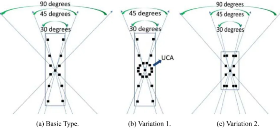
Figure 6 illustrates the concept of the proposed Rx an- tenna for seven concurrent OAM modes transmission in- cluding OAM modes −3,−2,−1, 0, 1, 2, and 3. We use a four-antenna-element set to receive a pair of OAM modes of which absolute values are identical and sign differ from each other such as OAM mode 1 and−1. We also use an antenna at the center for the OAM mode 0. In Fig. 5(a), the outermost, middle, and innermost four-antenna-element sets are respectively for OAM mode 3 and−3, 2 and −2, and 1 and−1. Four antenna elements in each set are located equidistant from the center and form an “X” type configura- tion. The angles of the two upper antenna elements of each set are respectively 30, 45, and 90 degrees. The angles of the two lower antenna elements of each set are the same as those of the upper ones. Note that such angles become narrower as the number of OAM modes increases. Therefore, contrary to the UCA case, the necessary area to capture the higher OAM modes does not increase by the power of two in its radius.
4.2 OAM Beam Separation
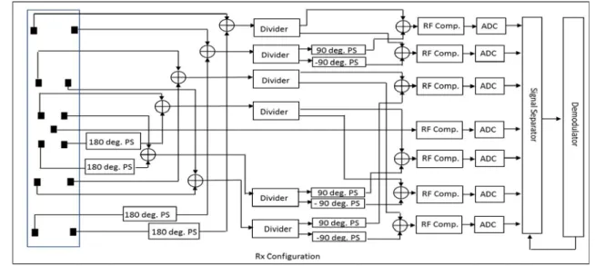
With the presented Rx antenna configuration, OAM beams are separated by analog cancellation followed by digital can- cellation. Referring to Fig. 7, we explain the details on the beam separation, which consists of the following three steps.
•Step 1) Analog Odd and Even OAM Modes Separation:
Diagonally located antenna elements in each four-antenna- element set are combined by either an equal-phase or reverse- phase combination using 2-to-1 analog combiners. Before the combinations, among the four-antenna-element sets in- stalled for odd OAM modes, both of the two antenna ele- ments at the bottom are first inserted to the 180 degree phase shifters as shown in Fig. 7. Since phase differences of even (odd) OAM beams at diagonally symmetric two antenna ele- ments respectively yield either 0 degrees or 180 degrees with identical intensities, equal (reverse) phase combinations of them cancel out all odd (even) OAM modes’ signals. With these equal-phase or reverse-phase combinations, combined outputs can to bear only either odd or even OAM modes.
•Step 2) Analog Extraction of each OAM Mode:
In this step each OAM mode is extracted using dividers, 90 and−90degree phase shifters, and combiners. We will ex- plain this step using an example of the extraction of OAM modes −3 and 3. Two reverse-phase combined outputs from the outermost four-antenna-element set contain only odd OAM modes (i.e., OAM mode−3,−1, 1, and 3) while even OAM modes’ signals are cancelled out.
Each of the two combined outputs is again divided into two signals by a 1-to-2 divider. One output of the two dividers is inserted into the 90 and−90degree phase shifters.
The outputs of these phase shifters are respectively combined again with the output of the other two dividers as shown in Fig. 7. These combined signals respectively yield OAM modes −3 and 3 containing some interference from OAM modes−1and 1. Since the intensities of OAM modes−1 and 1 are small at the outermost location we temporarily ignore them. However, these interferences are resolved by digital processing in step 3. Figure 8 shows a conceptual example to extract OAM mode 3.
Fig. 7 Configuration of Rx device using proposed Rx antenna.
Fig. 8 Conceptual example of OAM signal separation (OAM mode 3):
(a) One output of the reverse-phase combination using two antenna elements among the outermost four-antenna-element set, (b) Output of 90 degrees phase shifter using another output of the reverse-phase combination using remaining antenna elements among the outermost four-antenna-element set, (c) Output of−90 degrees phase shifter using another output of the reverse- phase combination using remaining antenna elements among the outermost four-antenna-element set, and (d) Combined signal of (b) and (c) (OAM mode 3 is extracted).
OAM modes−1and 1 are similarly extracted using two reverse-phase combined outputs from the innermost four- antenna-element set. OAM modes−2 and 2 are similarly extracted using two equal-phase combined outputs from the four-antenna-element set in the middle. OAM mode 0 ex- traction is directly obtained from the antenna element at the center since all OAM modes disappear other than OAM mode 0 at the center.
•Step 3) Digital Pruning of each OAM Mode:
Each of the OAM mode signals extracted in the previous step is further pruned by digital signal processing such as succes- sive interference cancellation (SIC) or MIMO equalization.
Remembering the previous statement on the beauty of OAM multiplexing that does not need complex signal processing,
this step may sound contradictory. Nevertheless, the signal processing complexity for this step is still tolerable since the proposed method does not need full channel interfer- ence cancellation. Precisely, the digital cancellation can be done by block diagonal matrix calculation rather than full matrix calculation. Also, more importantly, the number of necessary DACs and ADCs is still based on the number of streams rather than on the number of antenna elements.
Thus, we can still enjoy the advantages of OAM multiplexing that can reduce circuit complexity and corresponding power consumption. In addition, step 3 can be skipped when the residual interference after step 2 is negligible, or it can be intentionally skipped to reduce the complexity. The effect of skipping this step is evaluated in Sects. 6 and 7.
4.3 Variations of Reception Antenna Design
So far we have explained the usage of four-antenna-element sets (Basic Type, Fig. 6(a)). Some variations can also be considered. For example, it is possible to use both UCA and four-antenna-element sets (Variation 1, Fig. 6(b)). In this case, lower OAM modes including OAM modes−1, 0, and 1 are extracted by a UCA while higher OAM modes including OAM modes−3,−2, 2, and 3, are extracted by the proposed method.
It is also possible to allocate the outermost four-antenna- element set closest to the middle one as long as the angle conditions are satisfied (Variation 2, Fig. 6(c)). Although this case is not optimum for OAM modes−3and 3, signals can be captured in the high SNR region while maintaining the height of the proposed antenna in a reasonable range.
The performance of this antenna is discussed in Sect. 7.
In all cases, it is also possible to use the antenna ele- ment at the center to extract OAM mode 0 to prevent mode dependent performance.
5. Proposed Rx SNR Enhancement Methods
5.1 Usage of Gaussian Beams (Method A)
This subsection presents our first Rx SNR enhancement method using multiple Tx UCAs. We propose to use (La- guerre) Gaussian beams as OAM mode carriers. In contrast to OAM-carrying beams generated by a single UCA that has many harmonics of their peak intensities, Gaussian beams do not have harmonics of peak intensities[51]. This enables Rx SNR enhancement by preventing Rx energy dissipation due to harmonics of peak intensity.
From the perspective of array antenna technologies this may be considered a side lobe cancellation technology, and some other array antenna beam forming technologies can also be used as Rx SNR enhancement methods. However, our concern is not only such side lobe cancellation but also the generation of beams that carry OAM modes. We choose Gaussian beams since it is known that they can carry OAM modes[53]. The fact that they can be generated by using multiple UCAs with reasonable circuit complexity (as will be explained later) led us to focus on them. After reviewing Gaussian beams, we will describe a way to generate Gaussian beams carrying OAM modes by using multiple UCAs.
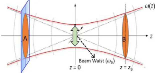
When the distance between the center of the beam (z =0, beam waist) and Rx is equal toz, the electric field distribution of the Gaussian beam with OAM modeLat Rx is given as follows:
uL(r, θ,z)=
√ 2 π(|L|!)*
,
√2r ω(z)+
-
|L|
ω0
ω(z)
·exp [
− r2 ω(z)2 −i
{ πr2
λ·R(z) +ΦG(z)−Lθ }]
(2) whereR(z)andω(z)are respectively the radius of the wave- front curvature and the Gaussian beam radius.
To avoid the confusion of the term, we call the peak intensity location of the OAM modes to be ring radius in this subsection. The ring radius of the OAM mode 2 equals to the Gaussian beam radius. They are respectively given by R(z)=(z2R+z2)/zandω(z) =ω0
√1+(z/zR)2whereω0
is the beam waist where the beam radius is minimized along the propagation direction. zRis the Rayleigh distance given by zR = (πω20)/λ. ΦG(z) is the Gouy phase that causes additional phase shifts and given by(1+|L|)·tan−1(z/zR).
We omitted descriptions of the physical meaning of these parameters because they are beyond the scope of this paper.
Details are given in[53].
Despite their capability to reduce the harmonics of peak intensity, Gaussian beams still have the characteristics of mode-dependent distinct peak locations. We consider the peak intensity location in each OAM of a Gaussian beam.
After calculating a partial differentiation equation in terms ofr, the peak intensity location of the OAM mode L, i.e., ring radius of the OAM modeL, is obtained as√
L/2·ω(z).
Fig. 9 Conceptual example of Gaussian beam generation.
Here,rindicates the radial distance from the Rx center in the polar coordinates. We also found that higher OAM modes tend to diverge more in this case and that the divergence is proportional to square root of the OAM mode.
Next, we will explain how we use multiple UCAs to generate Gaussian beams carrying OAM modes. For the simplicity, with referring to Fig. 9, we explain an example that Tx generates the identical beam size of Rx when the distance between Tx and Rx is2zB. In this case,uL(r, θ,zB) at location B in Fig. 9 is regenerated at the transmitter (loca- tion A in Fig. 9) anduL(r, θ,zB)is calculated from Eq. (2) by inserting concerned parameters such as each UCA’s ra- dius in the multiple UCAs and propagation distance. Then, we simply set our tunable parameters as calculated value of uL(r, θ,zB)at the transmitter. According to the Huygens–
Fresnel principle, electric field distribution of point sources can be calculated along the propagation[54]. We consider each Tx antenna element as a point source and apply this principle. Similarly, we can mimic a certain electric field distribution found in the middle of the propagation of un- der the condition that the area of the target electric field distribution to mimic is smaller than the Tx antenna size.
A close look at Eq. (2) gives us an insight that varying parameters arer andθand others are constants when zis fixed (z=zB). To further eliminate the varying parameters we choose multiple UCAs because the radiusris constant in each UCA. Since the only remaining varying parameter isθ, we can generate a Gaussian beam using phase shifters in the similar way as a Bessel beam generated by a single UCA. In summary, to generate the OAM mode L, antenna elements in each UCA are first set to an identical value that is de- terministically calculated from Eq. (2). Then these antenna elements are connected to phase shifters that giveL×360 degrees of phase rotation. Multiple beams carrying different OAM modes are independently generated and transmitted by the superposition.
The proposed method makes it possible to generate Gaussian beams carrying OAM modes using identical types of circuits, such as phase the shifters and combiners used in the case of beam generation by a single UCA. In prac- tice, mismatch in mimicking the electric field distribution of the Gaussian beam may occur when the number of antenna elements in the multiple UCAs is insufficient. Discussion regarding this is included in the evaluation section.
Fig. 10 Conceptual example of the usage of the dielectric lens.
5.2 Usage of a Dielectric Lens (Method B)
This subsection presents our second Rx SNR enhancement method using a dielectric lens by exploiting optical imaging theory[55],[56]. We explain the method on the basis of a single UCA for simplicity by extending our previous work [57],[58]. However, the usage of a single UCA and multiple UCAs are both possible.
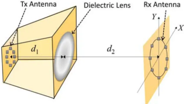
Figure 10 shows the concept of the proposed antenna with a dielectric lens configuration. Tx and Rx antennas are installed on planes perpendicular to the z-axis and their centers lie on the z-axis, as in previously made assumptions.
The dielectric lens installed between Tx and Rx UCAs constructs an optical imaging system. The transmitted beams carrying OAM modes are projected onto the Rx side as a “real image”. This approach seems simple but directly resolves problems associated with the Rx SNR degradation by the harmonics of peak intensities. In an ideal case where the aperture of the lens is infinite, the beam radius at the Rx size is calculated using the well-known lens formula given by 1/d1+1/d2=1/f. Here,d1,d2, and, f respectively denote the distance between the Tx UCA and lens, the distance between the Rx UCA and lens, and the focal length.
Now we turn into the practical case in which the aperture of the lens is finite. To derive the electric field distribution at the Rx plane, we borrow the following well-known knowl- edge from optical imaging theory. It says that the electric field distribution of beams passing through a lens having a finite radius is given by the first order Bessel function of the first kind[56]. When this is used in our system, the electric field distribution at the Rx plane is obtained by the superpo- sition of the electric field formed by beams passing through the lens as below.
fRX(X,Y)=C·exp[ i{
π(X2+Y2)/λd2}]
·
∑M L=1
∑N n=1
[
exp{i(2πLn/N)} ·πR2· J1(R·rn(X,Y)) R·rn(X,Y)
] , (3) where M, N, and L are respectively the total number of OAM modes, the total number of Tx antenna elements, and the OAM mode. (X,Y)is the Cartesian coordinates on the
plane holding the Rx antenna elements. R, J1(·), andC are respectively the radius of the lens, the first order Bessel function of the first kind, and a complex constant contain- ing all relevant factors such as attenuation and phase shifts.
rn(X,Y)given below is obtained from the lens formula.
rn(X,Y)=(2π/λd1d2)
√
(d1X+d2xn)2+(d1Y+d2yn)2, (4) where(xn, yn)is the locations of thenthTx antenna element.
As with the previous Rx SNR enhancement method by using Gaussian beams, it is necessary to derive the peak intensity location of each OAM mode. In contrast to the previous Gaussian beam case, it is not trivial to find such a peak location analytically. This is due to the fact that solving the partial differentiation equation of Eq. (3) forms a nested partial differentiation equation because the Bessel function in Eq. (3) itself includes the partial differential equation. In- stead of the analytically deriving the peak intensity location of each OAM mode, we investigated the effectiveness of the lens usage in a simulation study. Although explicit analysis is not included in this paper, combined usage of two proposed Rx SNR enhancement methods is also possible.
6. Evaluation: Proof of Concept Experiment
To examine the feasibility of OAM multiplexing, we con- ducted proof of concept experiments. First, beams carrying OAM modes were generated using an unmodulated signal at 5.2 GHz. Their propagation was also investigated. Second, wireless communication experiments using QPSK and 16- QAM modulated signals at the same frequency band were conducted using our proposed antenna. Third, the effect of the intensity and phase mismatch between experiment and theory was investigated. Note that a horn antenna was used for the OAM beams generation and their measurement to clearly capture the intensity and phase distributions at the Rx plane. On the other hand, our proposed antenna was used for the wireless communication experiments to confirm the validity of the proposed method.
6.1 OAM Beams Generation and Propagation Experiments Three beams respectively carrying OAM modes 0, 1, and 2 were generated using a single Tx UCA at different times.
Precisely, an unmodulated signal 5.2 GHz was generated and fed into a 1-to-8 divider. The transmission power was 7 dBm.
The divider’s 8 outputs were then respectively connected to 8 tunable phase shifters. Each tunable phase shifter was connected to the antenna elements of the Tx UCA. By set- ting the phases of the tunable phase shifters, beams carrying OAM modes were independently generated. For example, we set the phases from 0 degree to 315 degrees by increasing them in 45 degree increment to generate OAM mode 1. This yielded 360 degrees of phase rotation. To capture the inten- sity and phase distributions at the Rx plane, we used a horn Rx antenna and a moving positioner. While transmitting the
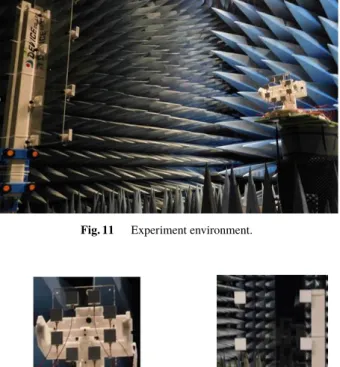
Fig. 11 Experiment environment.
Fig. 12 Tx and Rx antenna configurations, and radiation pattern.
generated OAM beam, we recorded the intensity and phase distribution at two dimensional grids of the Rx plane.
Figure 11 and the upper figure of Fig. 12(a) respectively show our experimental setup in the shielding room and the Tx UCA. The lower figure of Fig. 12(a) shows the radiation pattern of our Tx UCA. Considering practical limitations of our experimental environment, we set the distance between the Tx and Rx antennas to be around 235 cm (40.7λ). The diameter of the TX UCA was around 11.54 cm (2λ). The positioner was moved over a21×21square grid. One span of the grid was 5.77 cm (1λ) and the measured area at the Rx plane covered around 115.38 cm×115.38 cm. The center of the grid was set to be the peak intensity spot for OAM mode 0, while it was set to be the null points for OAM modes 1 and 2.
Measurement results of intensity and phase distribu- tions are shown in Fig. 13. Figure 14(a) shows average in- tensity distribution in terms of the distance from the center normalized to the peak intensity of OAM mode 0. We also measured the phase distributions circularly with a span of 15 degrees using OAM modes−1and 1. Figure 14(b) shows the measurement results, from which the following theoretical facts were experimentally confirmed.
•Intensity Distribution:
Fig. 13 Intensity and phase distributions (OAM modes 0, 1, and 2, inten- sity is normalized to the peak of OAM mode 0).
Fig. 14 Intensity and phase distributions (intensity is normalized to the peak of OAM mode 0).
The intensity distributions of OAM modes 0, 1, and 2 are respectively in good agreement with the zeroth, first, and second order of the Bessel function of the first kind. Null points of each OAM mode were observed as expected from the theory. Note that these values are normalized to the peak intensity of OAM mode 0. The second peak harmonics of the OAM mode 0 were also observed. The harmonics of peak intensities in OAM modes 1 and 2 were not seen due to the limited measurement area. Nevertheless, we argue that it may not be an exaggeration that harmonics of those OAM modes exist beyond our measurement area.
•Phase Distribution:
Phase distribution measurements also showed good overall agreement with the theory. The phases of OAM modes 0, 1, and 2 showed 0 degrees, 360 degrees, and 720 degrees of rotation. Some results deviating from the theory were found near the null points. We consider this is because measurements near the null points were unstable due to their low intensity. The phase rotation of OAM modes −1and 1 also showed good agreement with the theory within an allowable mismatch range. The effect of this mismatch is discussed in Sect. 6.3.
6.2 Modulated Signal Transmission Using OAM Beams This subsection describes the results obtained in a wireless communication experiment using modulated signals. Ex- cept for the Rx antenna, the experimental environment was the same as that used in previous experiments. Instead of
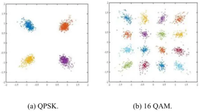
Fig. 15 Constellation map of modulated signals at the receiver.
using a horn antenna we used our proposed antenna shown in Fig. 12(b). The width and height of the Rx antenna were respectively 29 cm and 70 cm. QPSK and 16-QAM modula- tions were used for both uncoded and coded (1/2 rate LDPC) cases. The OFDM (orthogonal frequency division multi- plexing) was carried out with 64 subcarriers over a 20 MHz signal bandwidth. Among them 16 subcarriers are used.
Due to the practical limitations of the experimental setup, this experiment was conducted using a single stream while varying the OAM mode among−2, 1, 0, 1, and 2. The OAM multiplexing was evaluated by combining these single stream signals by offline processing. The transmitted signal of each stream is generated by an arbitrary waveform genera- tor (AWG) and transmission power is set to be the maximum of the AWG, i.e., 10 dBm.
Figures 15(a) and 15(b) respectively show the constel- lation mapping of QPSK (quadrature phase shift keying) and 16-QAM (quadrature amplitude modulation) signals.
Their EVM (Error Vector Magnitude) values were respec- tively 14.18% and 13.5% in the case of the OAM mode 1, and 14.3% and 15.65% in the case of the OAM mode 2.
Corresponding Rx SNRs calculated from EVM values were respectively 16.97 dB and 14.79 dB in the case of the OAM mode 1, and 16.89 dB and 13.51 dB in the case of OAM mode 2. These results validate the feasibility of wireless transmission by OAM multiplexing.
Note again that the above results are proof-of-concept level results. Further study is necessary regarding factors such as whether OFDM is optimum or not, the number of subcarriers, and the optimum modulation levels for each OAM mode.
6.3 Effect of Intensity and Phase Mismatch between The- ory and Experiment
To investigate the effect of the intensity and phase mismatch between theory and experiment, we first derived mismatch distributions by reusing our previous experimental results shown in Fig. 13. Figure 16 shows the derived distributions.
Prior to the investigation, we resolved the issue regard- ing the existence of large mismatches such as the 10 dB of intensity and 30 degrees in Fig. 16. Indeed, they are found near null points of each OAM mode. Since the intensity itself is low near the null points, the effect of such large
Fig. 16 Distribution of mismatch between experiment and theory.
Fig. 17 Performance evaluations.
mismatches is marginal. For example, the intensity of OAM mode 2 is 37 dB less than that of OAM mode 0 at the center.
Therefore, OAM mode 2 does not cause significant inter- ference to OAM mode 0 at the center even though a 10 dB mismatch in its intensity occurs.
In order to explore the effects of intensity and phase mis- matching, we compared the performance of an ideal AWGN channel and an experimentally modeled channel. To gen- erate the experimentally modeled channel, we respectively modeled the intensity and phase mismatch as Gaussian and uniform random variable by setting their standard deviations to the values given in Fig. 16. For example, when the radius was set to be 30 cm, the standard deviations of intensity mis- match for OAM modes 0, 1, and 2 were respectively set to be 2.8, 0.4, and 1.7 dB.
Figure 17(a) shows the results of such comparisons for an uncoded case when OAM modes 0, 1, and 2 were used.
The width and height of the proposed antenna were respec- tively set to 41 cm and 98.9 cm. These correspond to the 29 cm radius in Fig. 16. The antenna in the center was used for OAM mode 0. The transmission power was 7 dBm. The modulation was set to be BPSK. The distance between Tx and Rx was set to be 235 cm. For both the ideal AWGN and experimentally modeled channels, a simple diagonal equal- izer (EQ-diag) was used. Details for the EQ-diag are given in Sect. 7.2.
The bit-error-rate (BER) curves in Fig. 17(a) seem com- plex but show rather clear messages. First, BER perfor-
Fig. 18 Capacity comparisons.
mances for OAM modes 0 and 1 were very similar in both channels. This indicates that mismatching effects were neg- ligible. Second, BER performances for OAM mode 2 us- ing the experimentally modeled channel was slightly poorer (2 dB) than those using the ideal AWGN channel. The dif- ference shows the performance degradation effect due to mismatching.
Figure 17(b) shows the results of the coded (1/2 LDPC) case with the same setting with those of Fig. 17(a). It was confirmed that performance gap between the two channels was reduced compared to the uncoded case in Fig. 17(a).
This demonstrates that channel coding can overcome mis- matching between the theory and the experimental setting.
Surely, some redundancy is necessary for the channel cod- ing, but this might relax the strict requirements for the ex- perimental setup. We will reserve a precise study regarding this tradeoff for future work.
7. Evaluation of Rx Antenna Proposal
The new Rx antenna described in Sect. 4 was developed mainly to address mode dependency in performance. This tall, narrow antenna has the advantage of being able to cap- ture received signals far from the center. This is more ben- eficial when higher OAM modes are used. In this section we expand on this point with more general and thorough evaluations.
7.1 Capacity Comparisons
To show the mode dependency in performance, we con- ducted capacity comparisons in terms of the antenna radius by simulation. To ascertain the general mode-dependency trend, we started with the case where 5 OAM modes were used:−2,−1, 0, 1, and 2. To confirm the advantages of the proposed Rx antenna we then extended this to the case where 7 OAM modes were used: −3,−2,−1, 0, 1, 2, and 3. We assumed perfect signal separation among OAM modes for the proposed Rx antenna to focus on the achievable capacity.
The simulation settings for the 5 mode case were as fol- lows. The frequency band used was set to 5.2 GHz as it had
been in our experiments. The Tx UCA diameter was set to 11.54 cm (2λ) and the number of Tx antenna elements was set to 16. The modulation is set to be BPSK. The distance between Tx and Rx and Tx power were respectively set to be 235 cm and 10 dBm as in the previous experimental setting.
As with conventional methods, a single Rx UCA (hereafter
“UCA-1”) and a slightly modified version (hereafter “UCA- 2”) were used. Both UCA-1 and UCA-2 consisted of 8 antenna elements, but the latter also had an additional ele- ment in the center to make a total of 9. For the proposed Rx antenna (hereafter “Prop-1”), we used two four-antenna- element sets (Fig. 12(b)) with an additional element in the center (9 elements in total).
Figures 18(a), 18(b), and 18(c) respectively show capac- ities of each OAM mode and their sum capacity of UCA-1, UCA-2, and Prop-1. The horizontal axis of Figs. 18(a) and 18(b) refer to the radius of their UCA. The horizontal axis of 18(c) refers to the radius of the innermost four-antenna- element set of Prop-1. The width of Prop-1 is obtained by multiplying√
2by the radius. Its height is obtained by multiplying 2.414 (1/tangent (22.5 degrees)) by the width.
The capacity of each OAM mode in Fig. 18(a) shows typical mode-dependency. The maximum sum capacity is achieved when the antenna radius is about 30 cm. It de- creases when the antenna radius becomes larger than 30 cm because the intensity of OAM mode 0 approaches its null point. Due to the distinct antenna radius for the peak ca- pacity of each OAM mode, there is always loss in the max- imum capacity. The antenna size at the maximum capacity is60×60cm and its area is 0.36 m2in this case.
The capacity of UCA-2 is similar to that of UCA-1 except for OAM mode 0, which is always received by the antenna elements at the center. Therefore, the capacity of OAM mode 0 remains the same regardless of antenna size.
The maximum sum capacity of UCA-2 is obtained when the antenna radius is 48 cm. At this capacity the antenna size is 96×96cm and its area is around 0.92 m2.
The capacity of Prop-1 shows its maximum when the antenna radius is around 30 cm. This corresponds to the 42.4×102.4cm of the tall, narrow antenna. Its area is
Fig. 19 Performance evaluation of interference cancellation methods.
0.43 m2. It was confirmed that the proposed antenna yielded higher maximum capacity while the necessary antenna size was significantly smaller than that for the conventional method.
It might be argued that the maximum capacity can be increased by using multiple Rx UCAs for the conventional method. For example, antenna radii of close to zero for OAM mode 0, 40 cm for OAM modes−1and 1, and 60 cm for OAM modes−2and 2 yield increased maximum capacity for UCA-1. Likewise, the maximum capacity of UCA-2 can be increased when using multiple Rx UCAs with radii of 40 cm for OAM modes−1and 1 and 60 cm for OAM modes
−2and 2. However, in both cases the antenna size becomes 120×120cm and its area is 1.44 m2 while the increased maximum capacity is very similar to that of Prop-1. From the above we reconfirmed that the proposed Rx antenna is beneficial in terms of both antenna size and capacity.
Next, we consider the 7-mode case where the advan- tages of the proposed Rx antenna are more eminent. To prevent unnecessary increase in antenna size, we used the proposed antenna variation-1 illustrated in Fig. 6(b) which consists of 13 antenna elements (hereafter “Prop-2”). Fig- ure 18(d) shows the capacity comparisons between UCA-2 and Prop-2 in terms of the antenna radius. Here, to achieve a fair comparison with respect to the Rx antenna gain, we as- sumed the UCA-2 consists of a UCA of 12 antenna elements and an additional antenna element in the center (13 elements in total).
Due to the maximum capacity location of OAM modes
−3 and 3 being farther from the center, the antenna radius at the maximum capacity is around 52 cm for UCA-2. The antenna size at the maximum capacity is104×104cm and its area is around 1.086 m2 in this case. On the other hand, the maximum capacity is obtained when the antenna radius is around 38 cm. This corresponds to53.7×129.7cm and its area is 0.69 m2. In this 7-mode case, we confirmed the proposed Rx antenna had similar merits in terms of capacity and size. The following subsection uses the antenna radius of 38 cm to further study the superiority of the proposed methods.
7.2 Evaluation of Signal Separation Methods for the Pro- posed Rx Antenna
We analyzed the capacity of the proposed antenna by as- suming the perfect signal separation given in the previous subsection. If the complexity for signal separation is too high, the advantages of the proposed antenna are lessened and another tradeoff should be considered. This subsection discusses OAM mode separation methods considering their complexities.
We considered three separation methods, namely, the use of a simple diagonal equalizer (EQ-diag), a zero-forcing equalizer (EQ-ZF), and a SIC equalizer (EQ-SIC) for 7- mode case. After the analog extraction of each OAM mode (Step 2 in Sect. 4.2), one of these methods was applied.
We assumed that channel information would be available by pilot transmission or other typically used channel estimation methods.
EQ-diag does not conduct a digital interference cancel- lation process but directly performs the decoding processing using the extracted OAM signals obtained by an analog can- cellation process. EQ-ZF and EQ-SIC respectively conduct MIMO equalization based on ZF and SIC by digital signal processing. EQ-ZF and EQ-SIC respectively conduct singu- lar value decomposition (SVD) and QR decomposition while EQ-diag simply conducts scalar-value division. Despite the O(n3) complexity of EQ-ZF and EQ-SIC, overall complex- ity might not be significant as long as the channel does not change rapidly. Once SVD or QR decomposition has been done, the same value can be used repeatedly for a relatively long coherent time. If the usage scenario of OAM multi- plexing is taken into account, where the channel is static or slowly varies, the overhead for the channel estimation and the calculation cost will be tolerable.
Figure 19 shows the BER comparisons between EQ-ZF and EQ-diag when the horizontal antenna size is set to be 38 cm. The modulation is set to be BPSK. The distance be- tween Tx and Rx was set to be 235 cm. We did not display the EQ-SIC results because they are very similar to those of EQ-ZF. For UCA-2, EQ-ZF and EQ-diag yield the same per-
Fig. 20 Some extensions of the evaluations.
formance for all OAM modes since the orthogonality among OAM modes is maintained. On the other hand, the per- formances of EQ-ZF and EQ-diag in Prop-2 were different except for OAM mode 0. This is because the residual in- terferences are cancelled in EQ-ZF but are not cancelled in EQ-diag.
The performance gap between EQ-ZF and EQ-diag does not seem to be trivial. In particular, it is 9 dB in OAM modes−3and 3. We investigated the effect of channel cod- ing (1/2 LDPC) as a way to reduce the gap and found that was able to do so. For example, the performance gap between EQ-ZF and EQ-diag was reduced to less than 3 dB. This pro- vides us the possibility of reducing the digital cancellation step (Step 2 in Sect. 4.3) for the OAM signal separation when the channel coding is appropriately applied. This is feasible in a practical sense since channel coding is used in almost all wireless transmission technologies.
7.3 Effects of Interleaving, Power Compensation, Modula- tion Level, and Tx Antenna Size
We investigated the effectiveness of other common tech- niques such as interleaving and power compensation that might enable the mode dependency to be suppressed. Also brief study regarding the modulation level is done using 16 QAM. A 7-mode case was studied with the same simulation setting given in the previous section.
The effect of interleaving is given in Fig. 20(a). The interleaving was done by applying the channel coding (1/2 LDPC). The channel coding was conducted using a sin- gle stream. Then a coded signal was converted to parallel streams and transmitted using multiple OAM modes. By do- ing so, the interleaving effect was obtained without inserting additional interleaving and de-interleaving functions.
In the UCA-2 case, it is notable that 9 dB enhancement was achieved. Although the UCA-2 still showed poorer per- formance than the proposed Rx antenna, the interleaving with UCA-2 might also be a practical solution when the pro- posed antenna cannot be deployed. In the Prop-2 case, the best performance enhancement was achieved when both in-
terleaving and EQ-ZF were applied. Another notable point is that interleaving significantly improves performance when EQ-diag is used. This shows the feasibility of applying the proposed Rx antenna without implementing a signal sepa- ration method when proper channel coding and interleaving are used.
The effect of power compensation is shown in Fig. 20(b). We assumed power compensation was done by a Tx using the channel information and power compensation performed in a zero forcing manner. The results we obtained were similar to those obtained in the abovementioned inter- leaving cases, although there was slight overall performance degradation. This indicates that interleaving might be prefer- able because it does not need channel information at the Tx side.
The evaluation of the usage of the 16 QAM is shown in Fig. 20(c). It shows the BER results of OAM modes 3. Simulation settings are same other than the modulation level. In contrast to the previous ones, results obtained by EQ-diag show the error floor in both uncoded and coded cases while those obtained by EQ-ZF still show the enhanced performance comparing to the conventional method. In this case, EQ-ZF is necessary and digital cancellation step (Step 2 in Sect. 4.3) cannot be skipped.
Finally, we show the effect of Tx antenna size on the maximum capacity and corresponding antenna size that yields maximum capacity. As described in Sect. 3.4, the beam divergence becomes smaller as the Tx antenna size increases. Correspondingly, the necessary Rx antenna size becomes smaller when a larger Tx antenna is used. The results given in Fig. 20(d) confirm these facts. Although the values of maximum capacity and corresponding antenna area vary depending on the Tx antenna size, the trend of the re- sults was the same as in the studies described in the previous sections. In other words, the proposed antenna yields better maximum capacity with small antenna area even though the Tx antenna size varies.
Note that these results we obtained might not be the general trend for all cases. In future work we plan to further study optimum channel coding rates, modulation level, and
power pre-compensation methods for various cases, as well as the tradeoff issues described in Sects. 6.3 and 7.2.
8. Evaluation of the Rx SNR Enhancement Methods So far the frequency band of 5.2 GHz has been used for the proof of concept experiments and performance evaluation of the proposed Rx antenna. In this section we provide eval- uation results obtained by simulations for two Rx SNR en- hancement methods for wireless transmission over 60 GHz.
Here, we assumed the perfect coaxial alignment between Tx and Rx antennas.
8.1 Rx SNR Enhancement Method A
We will first show the feasibility of Gaussian beam gener- ation by using multiple UCAs when the distance between Tx and Rx is 30 m. Figure 21(a) shows the generated beam transition from the Bessel beam to the Gaussian beam as the number of UCAs and their antenna elements increases.
The left and right columns respectively show the intensity and phase of generated beams for OAM mode 1. Figures of the first and second rows respectively show Bessel beams generated by a single UCA consisting of 8 and 16 antenna elements. As stated previously, intensity peak harmonics were observed.
On the other hand, figures of the third and fourth rows respectively show Gaussian beams generated by two and four UCAs, each UCA consisting of 16 antenna elements. The residual harmonics of intensity peaks can be seen in the figures of the third row while a clear Gaussian beam with- out harmonics can be seen in the figures of the fourth row.
These figures confirm that the necessary number of antenna elements to generate Gaussian beams is the order of several tens. Since it is common for antennas to have this many elements, it can be argued that our idea of Gaussian beam generation using multiple UCAs is practical and feasible.
Comparisons of Rx SNR between the Bessel beam gen- erated by a single UCA and the Gaussian beam generated by multiple UCAs are shown in Fig. 21(b). The radius of the single UCA was set to be 30 cm (60λ). To generate the Gaussian beam, we used four concentric UCAs. Each consisted of 16 antenna elements and their radii were respec- tively set to be 7.5 cm (15λ), 15 cm (30λ), 22.5 cm (45λ), and 30 cm (60λ). Two cases of Rx antenna sizes of which radius respectively were 30 cm (60λ) and 40 cm (80λ) were investigated. The target distance for mimicking the electric field was set to be 30 m. In other words, we used the four UCAs to regenerate the electric field of the Gaussian beam at 30 m distance. OAM modes−2, −1, 0, 1, and 2 were generated for both Bessel and Gaussian beams. In all OAM modes, we were able to confirm that the Rx powers of the Gaussian beams were stronger than those of Bessel beams because power dissipation by the harmonics is mitigated.
We also conducted BER performance comparisons be- tween the OAM signals generated by the Bessel beams and those generated by the Gaussian beams. Figure 22 shows
Fig. 21 Comparisons of beam generation and Rx Power between Gaus- sian and Bessel beams.
Fig. 22 Evaluation of Rx SNR enhancement method A.
the results. The performances of the proposed method were superior to those of the conventional methods. This is also mainly due to the fact that power dissipation by the harmon- ics is mitigated in the case of Gaussian beams.
These results enabled us to confirm that the proposed method can generate a Gaussian beam carrying OAM modes.
More importantly, they enabled us to confirm that the pro- posed Rx SNR enhancement method is feasible.
8.2 Rx SNR Enhancement Method B
In this subsection we report how we investigated the per- formance of our second Rx SNR enhancement method, one which uses a lens by setting the distance between Tx and Rx from 8 m to 20 m. In order to validate the effectiveness of the proposed method, we compared beams generated by a conventional UCA with those generated by another UCA equipped with a lens (hereafter “lens-UCA”). The radii of the conventional Tx UCA and lens were set to be 15 cm (30λ) while the radius of the UCA in the lens-UCA was set to be 0.75 cm (1.5λ). The radius of the Rx UCA is set to be 15 cm (30λ) for the proposed method and 10 cm (20λ) and 15 cm (30λ) for the conventional method.
All UCAs consisted of 16 antenna elements other than
Fig. 23 Evaluations of Rx power.
the case of the conventional method of which Rx radius is 10 cm (20λ). In this case we used an additional antenna at the center to receive the signal of the OAM mode 0 to reduce the mode dependency. The distance between the Tx UCA in lens-UCA and the lens was 40 cm (80λ). The distance between Tx and Rx antenna was set to be 8 m. This lens-UCA yields an optical imaging system with 20-power magnification.
We first evaluated Rx power comparisons. Figure 23(a) shows the Rx intensity distributions in terms of the distance from the Rx center for both UCA and lens-UCA cases. These are respectively obtained by using Eqs. (1) and (3). We also inserted the penetration loss of the lens (10 dB) to the com- parison considering the penetration loss of other materials measured at 60 GHz [59]. The penetration losses of the glass, Plexiglas, and brick wall were respectively measured to be 4.3, 8.6, and 14.7 dB in[59]. The Rx power of the lens- UCA is stronger than that of the UCA for all OAM modes.
We also observed that the peak intensity location becomes far from the center as the number of OAM modes increases in both cases. For the lens-UCA, this is due to the finite size of the lens as stated in Sect. 5.2.
We also evaluated the effect of the Rx antenna offsets.
Although we used an optical imaging system, it is likely that the Rx antenna was not precisely located at the target loca- tion. In such cases, the Rx SNR might not be improved as much as the perfect precision case. Figure 23(b) shows the effect of such offsets. It can be seen that the peak inten- sity values become smaller and the peak intensity locations become farther from the center as the offsets increase. How- ever, the peak intensity degradation is relatively benign when we allow the usage of a larger Rx antenna. This tells us that even if the Rx antenna is not precisely located, the OAM signals’ Rx SNR can still be captured as long as a larger Rx antenna is used.
We also conducted BER performance comparisons be- tween the conventional UCA and lens-UCA. Figure 24 shows the results. They confirm that both a lens-UCA with perfect distance precision (on the basis of the lens formula) and
Fig. 24 Evaluation of Rx SNR enhancement method B.
also those with offsets show performance superior to that of the conventional UCA. This demonstrates the effectiveness of the proposed method in terms of Rx SNR improvement.
The method’s practicality is also confirmed from the results obtained for the lens-UCA with offset.
9. Discussion
Here we will discuss some important issues that are not directly mentioned in this paper but necessarily concern end- to-end wireless communication.
The first one is how to deal with the multipath chan- nel and how to conduct corresponding channel estimation and equalization. In particular, we focus on a LOS channel with multipath where not only dominant path but also non- negligible non-dominant paths exist. The first approach to dealing with such multipaths is simply relying on channel coding while skipping channel equalization. OAM multi- plexing is still possible with the use of strong channel cod- ing. This approach maintains the main advantage of OAM multiplexing, i.e., reduction of digital signal processing com- plexity at a small sacrifice in performance. The second ap-