Human capital externalities in Indonesian cities

(1)

Human capital externalities in Indonesian cities

著者 Hashiguchi Yoshihiro, Higashikata Takayuki

権利 Copyrights 日本貿易振興機構（ジェトロ）アジア

経済研究所 / Institute of Developing

Economies, Japan External Trade Organization (IDE‑JETRO) http://www.ide.go.jp

journal or

publication title

IDE Discussion Paper

volume 672

year 2017‑07

URL http://hdl.handle.net/2344/00049238

(2)

INSTITUTE OF DEVELOPING ECONOMIES

IDE Discussion Papers are preliminary materials circulated to stimulate discussions and critical comments

Keywords: Human capital externalities, urban areas, plant-level data, Indonesia JEL classification: E24, J24, J30, L60, O40

* Institute of Developing Economies-JETRO. E-mail: [email protected]

+ Institute of Developing Economies-JETRO. E-mail: [email protected]

IDE DISCUSSION PAPER No. 672

Human Capital Externalities in Indonesian Cities

Yoshihiro HASHIGUCHI^* and Takayuki HIGASHIKATA⁺

July 2017

Abstract

Using Indonesian plant-level manufacturing data for 1996 and 2006, this study estimates the external benefits of human capital investment. The external benefits are identified from the relationship between plant-level wages and city-level human capital stock, after controlling for workers’ skill levels, plant fixed effects, and time-varying industry fixed effects. Our results suggest that the degree of human capital externalities depends on the size of the urban population, and that such externalities do not occur in cities that either too large or too small. In the case of the Indonesian manufacturing industry, evidence of human capital externalities is observed in cities with a population of between 500 thousand and 1,500 thousand.

(3)

The Institute of Developing Economies (IDE) is a semigovernmental, nonpartisan, nonprofit research institute, founded in 1958. The Institute merged with the Japan External Trade Organization (JETRO) on July 1, 1998.

The Institute conducts basic and comprehensive studies on economic and related affairs in all developing countries and regions, including Asia, the Middle East, Africa, Latin America, Oceania, and Eastern Europe.

The views expressed in this publication are those of the author(s). Publication does not imply endorsement by the Institute of Developing Economies of any of the views expressed within.

INSTITUTE OF DEVELOPING ECONOMIES (IDE), JETRO 3-2-2, WAKABA,MIHAMA-KU,CHIBA-SHI

CHIBA 261-8545, JAPAN

No part of this publication may be reproduced without the prior permission of the IDE-JETRO.

(4)

Human Capital Externalities in Indonesian Cities ^∗

Yoshihiro HASHIGUCHI

^†

Takayuki HIGASHIKATA

^‡

March 2017

Abstract

Using Indonesian plant-level manufacturing data for 1996 and 2006, this study estimates the external benefits of human capital investment. The external benefits are identified from the relationship between plant-level wages and city-level human capital stock, after controlling for workers’ skill levels, plant fixed effects, and time-varying industry fixed effects. Our results suggest that the degree of human capital externalities depends on the size of the urban population, and that such externalities do not occur in cities that either too large or too small. In the case of the Indonesian manufacturing industry, evidence of human capital externalities is observed in cities with a population of between 500 thousand and 1,500 thousand.

Keywords: Human capital externalities, urban areas, plant-level data, Indonesia JEL classification: E24, J24, J30, L60, O40

1 Introduction

Does the presence of workers with higher human capital make other workers more productive?

If true, to what extent do the “external” benefits have an effect on a macro economy? The externalities associated with human capital investment have received remarkable attention as a key element in explaining cross-country differences in economic development (Lucas 1988;

Romer 1990). In addition, since the degree of the externalities is related to the efficiency of public investment in education, this issue is crucial not only for academics, but also for policy makers.

It is argued theoretically that human capital externalities occur through the sharing of workers’ knowledge and skills via social interaction (Lucas 1988; Acemoglu 1996; Duranton and Puga 2004). Many scholars have attempted to find empirical evidence of the externalities using individual wage or firm-level production functions (Rauch 1993; Acemoglu and Angrist 2000;

∗This study is conducted as part of the project Analysis of Urbanization in Indonesia using village census data from 1999 to 2014 at the Institute of Developing Economies (IDE-JETRO). This study utilizes data constructed under the support of JSPS KAKENHI (Grant-in-Aid for Young Scientists. (B)) Grant Number 25871152.

†Institute of Developing Economies-JETRO. E-mail: yoshihiro [email protected]

‡Institute of Developing Economies-JETRO. E-mail: takayuki [email protected]

(5)

Conley et al 2003; Moretti 2004a; 2004b; Ciccone and Peri 2006; Rosenthal and Strange 2008;

Abel et al. 2012; Liu 2013). While most studies have found evidence of positive human capital externalities in developed countries, mainly in the United States and Europe, Ciccone and Peri (2006) found no evidence of such externalities. In addition, only a few studies, including Conley et al. (2003) and Liu (2013), have examined this issue for developing economies.

The magnitude of human capital externalities remains controversial and, hence, more empirical studies are required, particularly for developing economies.

In this study, we use Indonesian plant-level manufacturing data for 1996 and 2006 to examine the existence of human capital externalities. Our contribution is twofold. First, to the best of our knowledge, our work is the first to investigate this issue using Indonesian plant-level manufacturing data. The data is based on the annual survey of medium and large manufacturing establishments (Survei Industri Besar/Sedang: IBS) conducted by the Indonesian Central Bureau of Statistics (Badan Pusat Statistik: BPS). Although many studies have examined the determinants of productivity in Indonesian manufacturing using the IBS plant-level database (Todo and Miyamoto 2006; Suyanto and Bloch 2009; Hallward-Driemeirer and Rijkers 2013;

Widodo et al. 2014), few studies explored the relationship between human capital and wages or productivity. Furthermore, because the IBS plant-level data have many missing values for fixed assets, the number of plants decreases by more than half after removing records affected by these missing values.¹ Using total factor productivity (TFP), which typically relies on capital stock, could lead to a large loss of sample data, causing serious bias in the estimation results.

In addition, there is a fundamental difficulty in the estimation of TFP, referred to as the simul- taneity problem between flexible inputs (such as labor and intermediate inputs) and unobserved productivity (Ackerberg et al. 2015; Gandhi et al. 2016). Thus, there is currently no consensus on an effective method for estimating TFP. To avoid these problems, we exploit plant-level wage variation to identify the magnitude of human capital externalities.

Second, we identify cities (urban areas) following the OECD’s (2012) methodology of defining urban areas, which is comparable internationally.² As Rauch (1993) argued, urban areas within a country are the most appropriate regional units to use to identify human capital externalities, because these areas are presumably at the same stage of economic development.³ However, the definition of an urban area differs among countries, which means the choice of definition can influence estimations of human capital externalities significantly. For this reason, we refer to the OECD’s (2012) methodology of defining urban areas, and apply it to community- level (the lowest administrative unit) map information and population census data.

The remainder of the paper is structured as follows. Section 2 describes our empirical model and estimation strategy. Section 3 presents the data sources, and Section 4 reports our empirical results. Lastly, Section 5 concludes the paper.

1According to the data we used, the sample size reduces by 44.8% owing to missing values on fixed asset information.

2In this paper, we use the terms “cities” and “urban areas” interchangeably.

3Regions at a higher stage of economic development are likely to have a larger and more advanced physical capital stock, which may also be factors that increase wages and productivity. This is why it would be difficult to identify the effects of human capital externalities using regions at different stages of economic development.

(6)

2 Econometric framework

2.1 Model

Consider a plant p operating in city c and industry j in year t. The plant produces output (Yt,p∈(j,c)) using several types of workers with different levels of skill (s), as well as the other factors of production, such as land, capital, or intermediate inputs. The production function is of the Cobb-Douglas type:

Y_t,p∈(_j,c) =Ajct

X

shs jctL_t,s,p∈(_j,c) α

Z_t,p∈(j,c)^1−α , (1)

where 0 < α < 1 is a parameter, Ajct is the local total factor productivity (TFP), hs jct is the efficiency of workers with skills, Lt,s,p∈(j,c) is the number of workers with skill s, andZt,p∈(j,c)is the amount of other factors of production. The profit of this plant is given by

πt,p∈(j,c) = pjctYt,p∈(j,c)−X

s

ws jctLt,s,p∈(j,c)−rjctZt,p∈(j,c), (2) wherepjct is the local price of its output,ws jct is the local wage of workers with skill s, andrjct

represents the local price of the other production factors. In the competitive equilibrium, the first order condition for profit maximization yields the following wage equation:

ws jct = α(1−α)^1−α^α Ajct

pjct

rjct

!1/α

hs jct

≡ Bjcths jct

(3)

The local wage for workers with skill s depends on their skills hs jct and a composite local productivity effect Bjct (Combes et al. 2008; Combes and Gobillon 2015). Since our empirical analysis is based on plant-level observations, we rewrite Equation (3) to reflect the wage per worker for plant p, as follows:

w¯t,p∈(j,c) ≡ P

sws jctLt,s,p∈(j,c)

Lt,p∈(j,c) = Bjct

P

shs jctL_t,s,p∈(_j,c) Lt,p∈(j,c)

≡ Bjcth¯_t,p∈(_j,c),

(4)

whereL_t,p∈(_j,c)is the total number of people employed by plant p, ¯w_t,p∈(j,c) is the labor cost per worker of plant p, and ¯ht,p∈(j,c)is the weighted average of worker efficiency for plant p.

Our empirical analysis is based on Equation (4), which indicates that wage differences among plants can reflect differences in the skill levels of workers (¯h_t,p∈(j,c)), as well as productivity differences (Bjct) caused by local and industrial characteristics. Then, we investigate whether city and industry-level human capital agglomeration has a positive effect on productivity (Bjct). Noted that the productivity effect is a function of total factor productivity (Ajct), the price of outputs (pjct), and the price of non-labor inputs (rjct). These three variables can be influenced by local and industrial characteristics, implying that we cannot separately identify price and technology effects on productivity (Combes et al. 2008).

(7)

2.2 An econometric specification

In order to empirically examine the influence of human capital agglomeration on the local industry productivity (Bjct), we specify a skill term (¯ht,p∈(j,c)) and a productivity term. Our data are a two-year (1996 and 2006), plant-level, balanced panel data. The definition of a city and the industrial classification is discussed in Section 3. For ease of notation, in the remainder of the paper, we express p ∈(j,c) as p. First, we assume that the average worker efficiency for plant pis given by

log ¯hpt =βEpt+δp+εpt, (5)

where β is a parameter, Ept is the average years of education of workers, δp is a plant fixed effect, andεpt is a measurement error. Then,Ept is given by

Ept = L^N_pt Lpt

+6L^PR_pt Lpt

+9L^JH_pt Lpt

+12L^{S H}_pt Lpt

+14L^D3_pt Lpt

+16L^BA_pt Lpt

+19L^MD_pt Lpt

, (6)

whereLpt is total number of workers, and the other terms denote the number of workers who have not finished primary school (L^N_pt), and those who have completed primary school (L^PR_pt ), junior high school (L^JH_pt ), senior high school (L^{S H}_pt ), an associate (Diploma 3orProfesional ahli madya) (L^D3_pt ), a bachelor (L^BA_pt ), and a masters/doctoral education (L^MD_pt ).

The composite of local productivityBjct is assumed to be given by

logBjct = θH−jct+µjt+ηjct, (7) whereH−jct represents the degree of human capital agglomeration in citycoutside industry j, θdenotes the degree of human capital externalities,µjt is an industry×year effect, andηjct is a measurement error representing time-varying local and industrial unobservable characteristics.

We use the following two variables for the degree of human capital agglomeration in city c outside of industry of j:

H−jct ≡S highEdu−jct or AveEduYrs−jct, (8) whereS highEdu−jctis the share of at least some senior high school-educated workers among all manufacturing workers in cityc, with the exception of workers in industry j, andAveEduYrs−jct

is the average years of education of all manufacturing workers in cityc, with the exception of workers in industry j.

Combining Equations (4), (5), and (7), and taking the first difference to remove a plant effect δp, we obtain the following econometric specification:

∆log ¯wpt =β∆Ept+ ∆logBjct+ ∆εpt

∆logBjct =θ∆H−jct+ ∆µjt+ ∆ηjct. (9) The key parameter of this equation isθ, which captures the degree of human capital externalities occurring within a city across industrial sectors, but does not capture those occurring within a plant or within the same industry.

(8)

2.3 Econometric strategy

There are two main issues when estimating the degree of human capital externalitiesθin Equa- tion (9). The first is that the true value of∆logBjctis unknown because of the existence of the unobserved local endowments∆ηjct. The second is the endogeneity of human capital agglomeration∆H−jct. The following describes these two issues.

Dealing with an unobserved endowment variable: Two-step estimation

Substituting the second equation in Equation (9) into the first one, we can obtain a single es- timable wage equation. However, the single-step estimation creates large biases in the standard errors for the estimated coefficients of aggregate explanatory variables because we cannot separately specify local shocks (∆ηjct) and shocks at the plant level (∆εpt). Moreover, it does not allow for the correlation between plant characteristics (∆Ept) and∆ηjct, yielding a possible source of endogenous biases.⁴ On the other hand, the specification shown in Equation (9) takes into account possible correlations between∆Ept and∆ηjct, and allows us to control for the bias in the standard errors. This should lead to a more consistent evaluation on the degree of human capital externalities.

For the estimation of Equation (9), we use a two-step estimation procedure proposed by Combes et al. (2008). In the first step, we estimate∆logBjct using a city-industry-time fixed effect:

∆log ¯wpt =β∆Ept +XN_JC

j,c Dp jcαjc+ ∆εpt, (10)

whereDp jc is a dummy variable such that Dp jc = 1 if plant pbelongs to industry jand cityc, andNJC denotes the total number of pairs (j,c) observed in the plant-level panel data. The estimates ( ˆαjc ≡∆logˆBjct) are substituted into the second equation of Equation (9). Note that the subscriptt is removed fromPN_JC

j,c Dp jcαjcbecause our panel data have only two periods. Since the estimates have the sampling errorΨ^jct = ∆logBjct−∆logˆBjct, the second step specification is represented as

∆logˆBjct =θ∆H−jct+ ∆µjt+ ∆ηjct+ Ψjct

=θ∆H−jct+ ∆µjt+ejct, (11) where ejct = ∆ηjct + Ψjct. Although the covariance matrix of ejct is complex owing to the existence of the sampling error, this can be dealt with using the feasible generalized least- squares (FGLS) estimator proposed by Gobillon (2004) and Combes et al. (2008). Following these previous studies, we estimate the covariance matrix ofejct, and then calculate the FGLS estimates ofθusing the estimated covariance matrix.⁵

4For the detail of this estimation problems, refer to Moulton (1990), Combes, et al (2008), and Combes and Gobillon (2015).

5For the estimation procedure of the covariance matrix, refer to Gobillon (2004, pp. 5–6) and Combes et al.

(2008, p. 741).

(9)

Endogeneity of human capital agglomeration

The second issue with our estimation is the correlation between changes in human capital agglomeration in cityc, outside industry j,∆H−jct, and the error termejct in Equation (11). Plant- level panel data allow us to control for many time-invariant and time-varying factors that are likely to influence the human capital agglomeration. In our specification, all time-invariant effects are fully removed from the estimation equation by taking the first difference. This elim- inates a bias that might arise if geographic features such as social infrastructures, natural re- sources, or local climate attract productive firms, and/or if more productive firms self-select to locate themselves in cities with high human capital accumulation. In addition, changes in industry-specific productivity shocks (or business cycle) are absorbed by an industry × year effect∆µjt.

A heterogeneity that is not considered in our specification is a city×year effect (∆µct). This is a possible source of the endogeneity bias in the spillover effect of human capital agglomeration.⁶ Time-varying city-wide positive productivity shocks (e.g., the openings of an airport or freeway) are expected to improve all plants in a city, and may attract highly educated workers to the city. Consequently, there is a possibility of a correlation between a city×year effect and

∆H−jct.

Although our specification takes into account many possible sources of an endogenous bias in the OLS or FGLS estimates of the effect of human capital externalities, it remains possible that the estimate may include the influence of a time-varying city-wide productivity shock. To deal with this problem, we use an instrumental variable approach. Our instrument for ∆H−jct

is based on large plants closings, and we exploit the impact of the 1997 Asian Financial Cri- sis on the human capital accumulation. Assuming that the crisis is an exogenous shock to the Indonesian economy, we consider that cities where there are relatively many large plants that were forced out of business due to the crisis are expected to have lower rate growth of human capital accumulation, because larger firms are likely to employ more educated workers.⁷ Hence, closing large plants is expected to have a large impact on the changes in human capital accumulation∆H−jctin the city. Specifically, our instrumental variable is the share of all manufacturing workers employed in exiting plants during 1997–1999 in cityc, with the exception of plants in industry j:

S E xitEmp−jc= E xitEmp−jc

T otalEmp−jc

(12) where E xitEmp−jc is all manufacturing workers in city c, other than in industry j, that are employed by plants that exist in 1996 and closed during 1997–1999, and that have 300 or more workers. The denominatorT otalEmp−jc is all manufacturing workers from 1997 to 1999 that are employed by plants that exist in 1996 in cityc, other than in industry j. Our instrument is expected to have a negative effect on the changes in human capital accumulation.

6It is theoretically possible to add a city×year effect. However, this is not feasible in practice. Because our data are based on two-digit industrial classifications and the number of sectors is quite small, most of the sample variations inH−jctare at the city×year level.

7Based on plant-level balanced panel data using our empirical analysis, the correlation between the average years of education of workers within a plant and the log of the total number of workers is 0.312, which is significant at the 0.01% level.

(10)

3 Data description

Our main databases are 1996 and 2006 plant-level data on the Indonesian manufacturing industry, and 2000 population data of administrative village (community), which is the lowest administrative unit.⁸ The plant-level data are obtained from the annual survey of medium and large manufacturing establishments (IBS) conducted by the BPS. The IBS covers all manufacturing plants with 20 or more employees. Although the IBS is published annually, we use only the 1996 and 2006 databases because they include information on workers’ educational attainment.

In order to define urban areas (cities, in our empirical specification), we use the community- level population and area data. The population data are obtained from the 2000 population census (Sensus Penduduk 2000). The 1999 population data of the Village Potential Data Col- lection (PODES) database are also used if the 2000 population census data are not available in some places.⁹ The area of each community, needed to measure population density, is calculated using the community-level map information of the 2012Peta Digital database in the shapefileformat. The Peta Digital consists of 506 shapefiles, and each shapefile basically has one district-level map including community-level polygon data. Because almost all shapefiles in the Peta Digital use the format known as WGS84 geographic coordinate system, we covert the coordinates into the Universal Transverse Mercator (UTM) zone projection for Indonesia (DGN95-UTM) to calculate the community-level areas as precisely as possible.¹⁰ The 2012 Peta Digital map data are merged with the 1999 and 2000 population data by using information about historical transition of administrative communities from 1998 to 2013. According to the Peta Digital, the number of communities is 78,934 in 2012. 76,565 (97%) of them are matched with the 1999 and 2000 population database, and thus the matched samples are used to define urban areas.¹¹

Referring to the definition of OECD (2012), we compute urban areas as follows: (1) we select communities with a population greater than 1,500 per square km; (2) cluster these communities as an area if they have common borders; and (3) define the computed cluster with a population size greater than 100 thousand as an urban area. The Peta Digital map data is used to identify communities with common borders.

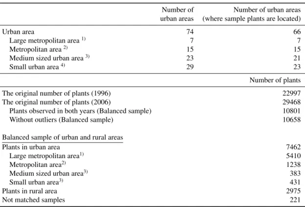
[– Table 1 –]

As shown in Table 1, the total number of urban areas is 74, and the total urban area is 145,345 square km, which covers approximately 7.6% of the total land area in Indonesia. The total urban population is about 62,872 thousand, which is approximately 30.5% of total popu-

8Indonesia’s administrative divisions are classified as follows: province (provinsi), regency/city (kabu- paten/kota), district (kecamatan), and community (desa/kelurahan).

9We use the 1999 PODES population data for 4,117 communities. Of these, 3,146 belong to Ache province, and the remaining communities are located in Papua and West Papua provinces (778 units) and North Maluku province (108 units), among others.

10There are 15 UTM zones commonly used for Indonesia. The WGS84 coordinate for each shapefile is converted into the coordinate of a UTM zone in which the center point of the shapefile is located.

11The number of unmatched communities is 2,369, and 38% of them belongs to West Sumatra province, fol- lowed by North Sumatra province (8.8%). These communities are outside the scope of this study.

(11)

lation in 2000. Table 1 also describes the number of manufacturing plants in 1996 and 2006.

The original databases of IBS 1996 and 2006 have 22,997 and 29,468 plants, of which 10,801 plants are observed in both years. After dropping outliers,¹² we have 10,658 plants, of which 7,462 are located in urban areas, and 2,975 are located in rural areas. The remaining 221 plants do not match the community-level population data.¹³

[– Table 2 –]

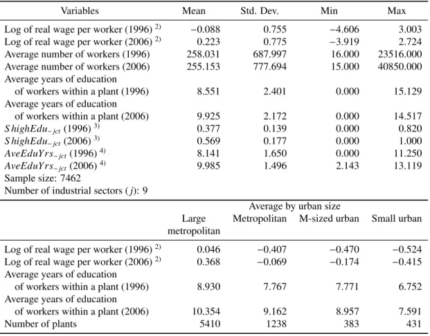
Our empirical analysis is based on the plant-level balanced panel data of urban areas. Ta- ble 2 describes the summary statistics of the variables. Wages are deflated by the district-level GDP deflator, normalized at the year 2000.¹⁴ The definition of average years of education within a plant is shown in Equation (6). The proxy variables for human capital agglomeration (S hingEdu−jct, AveEduYrs−jct) are constructed as follows. These two variables for 1996 and 2006 are based on the 1995 Intercensal Population Survey (SUPAS) and the 2006 National Socio-Economic Survey (SUSENAS), respectively. Both databases contain information on the number of workers with educational attainment by sector and by community. We extract the community-level data of workers located in the urban areas from these databases using community codes and names, and then construct the variables of human capital agglomeration by city (urban) and industry. The industrial classification is based on the two-digit Indonesian standard industrial classification (KLUI1990), and the number of manufacturing sectors (j) is nine.¹⁵

According to Table 2, the larger the urban size is, the higher is the wage per worker, indicating a possibility that plants operating in larger urban areas are more productive. On the other hand, larger urban areas also have higher average years of education of workers within a plant, implying that the higher wage in large urban areas may reflect the concentration of highly educated workers in those areas.

4 Estimation results

[– Table 3 –]

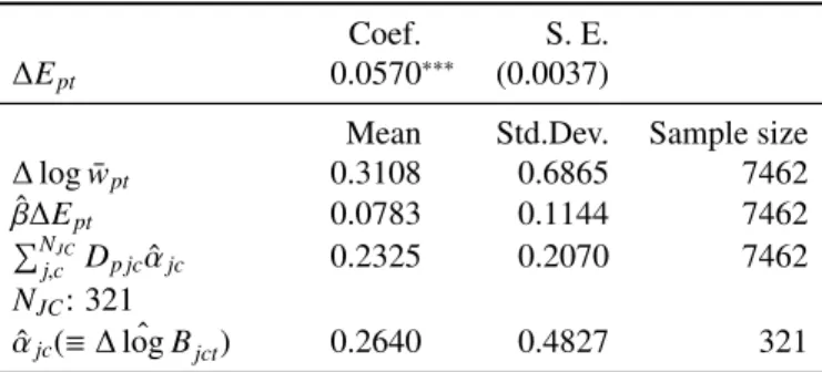
Table 3 reports the first-step estimation results of Equation (10). The estimated coefficient

12We remove the following plants: 1) plants with non-positive value of wages, number of workers, value-added, or output values; or 2) plants whose real wage per worker in 2006 is more than 1000 times or less than 0.001 the value in 1996.

13To merge the IBS plant-level data and the 2000 village-level population census data (SP), we use the 1996 community-level codes and names shown in the 1996 PODES database. Assuming that the community-level administration code of the 1996 IBS data is the same as that of the 1996 PODES data, we merge the 1996 IBS and the 1996 PODES databases. Since the 1996 PODES and the 2000 SP databases have the name lists of communities, we merge the 1996 IBS data and the SP data using these lists of communities.

14We construct the district-level GDP deflator based on the 1996 administrative divisions, where the number of districts is 294.

15The industrial classification differs between the 1995 SUPAS and the 2006 SUSENAS. The former is the two-digit base of the KLUI1990 classification, and the latter is the three-digit base of the KBLI2000 classification.

These are unified using the two-digit classification of KLUI1990.

(12)

of ∆Ept is 0.057 and significant, indicating that an increase in average years of education of workers within a plant leads to a 5.7% increase in the real average wage of a plant. The mean of∆log ¯wpt is 0.311, which is equal to the sum of the means of ˆβ∆Ept andPN_JC

j,c Dp jcαˆjc. The means of ˆβ∆Ept and PN_JC

j,c Dp jcαˆjc are 0.0783 and 0.2325, and hence, on average, 25.19% of total changes in real wages are explained by changes in average years of education of workers.

The remaining 74.81% is explained by changes in local and industrial characteristics.

[– Table 4 –]

Table 4 shows the estimation results of the second-step equation (11). The estimated coefficients of the human capital agglomeration (∆S highEdu−jct, ∆AveEduYrs−jct) are not statistically significant for both OLS and FGLS estimates. The 2SLS estimates are also insignificant, and have large standard errors. This is probably because, as shown in the results of first-stage regression, the instrument is weakly correlated with the endogenous variable. Our instrument is based on the share of workers employed in large plants that were forced out of business during the Asian Financial Crisis. We attempt to use other instruments based on the different definition of large plants, such as plants with over 100 workers, 300 workers, and 500 workers.

In addition, the share of plants, rather that of workers, is also used for the instrument. How- ever, these instruments are all weakly correlated with the endogenous variable, and lead to the large standard errors in the second-stage estimates. Finding more suitable instruments remains a problem.

Let us examine the OLS and FGLS estimates in Table 4. These estimates are all statistically insignificant, and all have large standard errors. This indicates that an increase in human capital agglomeration in a city, other than in industry j, does not improve the city’s productivity of industry j. This implies that there are no human capital externalities in the Indonesian manufacturing industry. Since large standard errors of estimates are likely to reflect the heterogeneity of coefficients, we estimate the coefficients of∆S highEdu−jct and∆AveEduYrs−jct

by urban size, using urban size dummy variables which are classified by the four categories of urban size: Large metropolitan, Metropolitan, Medium-sized urban, and Small urban areas.¹⁶ The definition of these categories is described in the footnote of Table 1.

[– Tables 5 and 6 –]

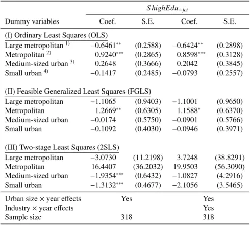
Tables 5 and 6 report the estimates of coefficients for each urban group. We find that Metropolitan area has positive and significant estimates of∆S highEdu−jct, while the OLS estimates of Large metropolitan are negative and significant. The other urban areas have statistically insignificant coefficients. The OLS and FGLS estimates of ∆AveEduYrs−jct by urban size remain insignificant (Table 6) . The 2SLS estimates in Tables 5 and 6 still have large standard errors, mainly because of the weak instrument problem. Thus, our estimates by urban size remain unstable owing to the large standard errors. However, according to the estimates of∆S highEdu−jct, it seems that the magnitude of human capital externalities depends on urban population size, and such externalities do not occur in cities that are either too large or too small.

16We also estimate the coefficients by two-digit industrial sector. However, almost all of these estimates are statistically insignificant.

(13)

In the case of the Indonesian manufacturing industry, evidence of human capital externalities is observed in cities with a population of between 500,000 and 1,500,000 (i.e., Metropolitan area). Based on the FGLS estimates of∆S highEdu−jctin the Metropolitan, an increase of one percentage point in the share of at least some senior high school-educated workers among all manufacturing workers in cityc, with the exception of workers in industry j, is associated with a 1.159–1.267% increase in productivity in cityc, industry j.

[– Figure 1 –]

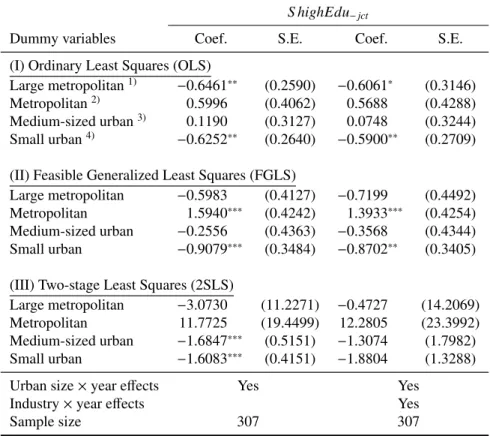
A concern with our estimation is that the standard deviation of∆logˆBjct is large, as shown in Table 3 and, hence, some outliers may influence the estimation results. Figure 1 shows the scatter plots of∆logˆBjct and∆logH−jct. The vertical axis is∆logˆBjct, and the horizontal axis is∆S highEdu−jctin panel (I), and∆AveEduYrs−jctin panel (II). The dotted lines show plus and minus three standard deviations from the mean. We consider samples above the dotted lines as outliers, and conduct the second-step estimation without these samples. Table 7 reports the estimation results. To save space, we show the estimates for∆S highEdu−jct only. Compared with the results of all samples, the OLS estimates of Metropolitan have relatively large standard errors and the coefficients are small and statistically insignificant. However, the FGLS estimates remain positive and significant, and the standard errors are smaller than those of the estimates using all samples. Therefore, outliers have little influence on our main findings.

[– Table 7 –]

5 Concluding remarks

Despite its importance to economic development, few studies have examined empirical evidence of human capital externalities for the Indonesian economy. Furthermore, while urban areas have been regarded as important and appropriate units from which to identify human capital externalities, existing studies have used different definitions of urban areas, depending on the countries of origin. Because changing the definition may influence the estimation of human capital externalities significantly, it is important to use an internationally comparable definition, and to investigate the effects of changing the definition.

This study analyzes the magnitude of human capital externalities using Indonesian manufacturing plant-level data for 1996 and 2006. We identify urban areas referring to the OECD’s (2012) methodology of defining urban areas, which is internationally comparable. Our first empirical results suggest that the magnitude of human capital externalities depends on urban population size, and such externalities do not occur in cities that are either too large or too small. In the case of the Indonesian manufacturing industry, evidence of human capital externalities is observed in cities with a population of between 500,000 and 1,500,000. According to the most plausible estimates, an increase of one percent point in the share of at least some senior high school-educated workers among all manufacturing workers in citycwith the exception of workers in industry jis associated with a 1.159–1.267% increase in productivity in city c, industry j.

(14)

Note that these findings are preliminary, and our empirical analysis has at least two problems that need to be solved. First, since we found that our instrument based on large plants closing owing to the Asian Financial Crisis has a weak correlation with the share of more highly educated workers in a city, finding more suitable instruments is necessary. Second, we should investigate to what extent the estimates of human capital externalities are affected by changes to the definition of urban areas. We need to address these remaining issues.

References

Abel, J. R., Dey, I., Gabe, T. M. (2012) Productivity and the density of human capital. Journal of Regional Science52(4), 562–586.

Acemoglu ,D. (1996) A microfoundation for social increasing returns in human capital accumulation.Quarterly Journal of Economics111(3), 779–804.

Acemoglu, D., Angrist, J. (2000) How large are human-capital externalities? Evidence from compulsory schooling laws. NBER macroeconomics annual15: 9–59.

Ackerberg, D. A., Caves, K., Frazer, G. (2015) Identification properties of recent production function estimators. Econometrica83(6), 2411–2451.

Ciccone, A., Giovanni, P. (2006) Identifying human-capital externalities: Theory with applica- tions. Review of Economic Studies73(2), 381–412.

Combes, P., Duranton, G., Gobillon, L. (2008) Spatial wage disparities: sorting matters! Jour- nal of Urban Economics63(2), 723–742.

Combes, P., Gobillon, L. (2015) The empirics of agglomeration economies. In: G. Duranton, J. V. Henderson and W. C. Strange, Eds, Handbook of Regional and Urban Economics, Elsevier, Vol. 5, 247–348.

Conley, T. G., Flyer, F., Tsiang, G. R. (2003) Spillovers from local market human capital and the spatial distribution of productivity in Malaysia. Advances in Economic Analysis & Policy 3(1),

Duranton, G., Puga, D. (2004) Micro-foundations of urban agglomeration economies. In: Hen- derson JV, Thisse JF (eds) Handbook of regional and urban economics, vol. 4. North- Holland, New York.

Gandhi, A., Navarro, S., Rivers, D. (2016) On the identification of production functions: How heterogeneous is productivity?

Gobillon, L. (2004) The estimation of cluster effects in linear panel models. Processed, INED.

Hallward-Driemeier, M., Rijkers, Bob. (2013) Do crises catalyze creative destruction? Firm- level evidence from Indonesia.Review of Economics and Statistics95(5), 1788–1810.

Liu, Z. (2013) Human capital externalities in cities: Evidence from Chinese manufacturing firms. Journal of Economic Geographyibt024.

Lucas, R. E. (1988) On the mechanics of economic development. Journal of Monetary Eco- nomics22(1), 3–42.

Moretti, E. (2004a) Estimating the social return to higher education: Evidence from longitudinal and repeated cross-sectional data.Journal of Econometrics121(1), 175–212.

Moretti, E. (2004b) Workers’ education, spillovers, and productivity: Evidence from plant-level production functions. American Economic Review94(3), 656–690.

Moulton, B. R. (1990) An illustration of a pitfall in estimating the effects of aggregate variables

(15)

on micro units.Review of Economics and Statistics72(2), 334–338.

OECD (2012) Redefining “Urban”: A new way to measure metropolitan areas. OECD Pub- lishing, Paris.

Rauch, J. E. (1993) Productivity gains from geographic concentration of human capital: Evi- dence from the cities. Journal of Urban Economics34(3), 380–400.

Romer, P. R. (1990) Endogenous technological change.Journal of Political Economy98(5) part 2, S71–S102.

Rosenthal , S. S., Strange, W. C. (2008) The attenuation of human capital spillovers. Journal of Urban Economics64(2), 373–389.

Suyanto, R. A. S., Bloch, H. (2009) Does foreign direct investment lead to productivity spillovers?

Firm level evidence from Indonesia. World Development37(2), 1861–1876.

Todo, Y., Miyamoto, K. (2006) Knowledge spillovers from foreign direct investment and the role of local R&D activities.Economic Development and Cultural Change55(1), 173–200.

Widodo, W., Salim, R., Bloch, H. (2014) Agglomeration economies and productivity growth in manufacturing industry: Empirical evidence from Indonesia. Economic Record 90(s1), 41–58.

(16)

Table 1: Number of urban areas and sample plants

Number of Number of urban areas urban areas (where sample plants are located)

Urban area 74 66

Large metropolitan area¹⁾ 7 7

Metropolitan area²⁾ 15 15

Medium sized urban area³⁾ 23 21

Small urban area⁴⁾ 29 23

Number of plants

The original number of plants (1996) 22997

The original number of plants (2006) 29468

Plants observed in both years (Balanced sample) 10801

Without outliers (Balanced sample) 10658

Balanced sample of urban and rural areas

Plants in urban area 7462

Large metropolitan area¹⁾ 5410

Metropolitan area²⁾ 1238

Medium sized urban area³⁾ 383

Small urban area³⁾ 431

Plants in rural area 2975

Not matched samples 221

Notes: Urban areas are calculated using the 2000 village-level population data.

1)Urban areas with population≥1500,000.

2)Urban areas with population 500,000–1500,000.

(17)

Table 2: Summary statistics¹⁾

Variables Mean Std. Dev. Min Max

Log of real wage per worker (1996)²⁾ −0.088 0.755 −4.606 3.003

Log of real wage per worker (2006)²⁾ 0.223 0.775 −3.919 2.724

Average number of workers (1996) 258.031 687.997 16.000 23516.000 Average number of workers (2006) 255.153 777.694 15.000 40850.000 Average years of education

of workers within a plant (1996) 8.551 2.401 0.000 15.129

Average years of education

S highEdu−jct(1996)³⁾ 0.377 0.139 0.000 0.820

S highEdu−jct(2006)³⁾ 0.569 0.177 0.000 1.000

AveEduYrs−jct(1996)⁴⁾ 8.141 1.650 0.000 11.250

AveEduYrs−jct(2006)⁴⁾ 9.985 1.496 2.143 13.119

Sample size: 7462

Number of industrial sectors (j): 9

Average by urban size

Large Metropolitan M-sized urban Small urban metropolitan

Log of real wage per worker (1996)²⁾ 0.046 −0.407 −0.470 −0.524 Log of real wage per worker (2006)²⁾ 0.368 −0.069 −0.174 −0.415 Average years of education

Average years of education

Number of plants 5410 1238 383 431

1)Number of sample plants observed in urban areas for both 1996 and 2006.

2)The real wage is the nominal wage divided by the district-level GDP deflator, normalized to 100 in the year 2000. The average of the deflator is 49.3 for 1996 and 165.2 for 2006. The unit of nominal wage is 1000 Rupiah.

3)This is the share of at least some senior high school educated workers among all manufacturing workers in cityc, with the exception of workers in industryj.

4)This is the average years of education of all manufacturing workers in cityc, with the exception of workers in industry j.

(18)

Table 3: Estimation results of Eq. (10)

Coef. S. E.

∆Ept 0.0570^∗∗∗ (0.0037)

Mean Std.Dev. Sample size

∆log ¯wpt 0.3108 0.6865 7462

βˆ∆Ept 0.0783 0.1144 7462

PN_JC

j,c Dp jcαˆjc 0.2325 0.2070 7462 NJC: 321

αˆ_jc(≡∆logˆ B_jct) 0.2640 0.4827 321 Note: Figures in parentheses are standard errors, clustered by district-level region. The asterisks^∗, ^∗∗, and ^∗∗∗ denote 10%, 5%, and 1% significance levels. NJC denotes the total number of pairs of industryjand citycobserved in the plant-level data.

Table 4: Estimation results of Eq. (11)

(1) (2) (3) (4)

(I) Ordinary Least Squares (OLS)

S highEdu−jct 0.1388 0.1312 (0.1914) (0.2068) AveEduYrs−jct

−0.0011 −0.0033 (0.0225) (0.0251) (II) Feasible Generalized Least Squares (FGLS)

S highEdu−jct

0.0924 0.0588 (0.276) (0.279)

AveEduYrs_−jct −0.0319 −0.0370

(0.0347) (0.0345) (III) Two-stage Least Squares (2SLS)

S highEdu−jct

−0.7637 −0.8814 (1.8980) (1.6278) AveEduYrs−jct

−0.0705 −0.0820 (0.1716) (0.1631) First stage

S E xitEmp−jc 0.2884 0.2858 3.1240 3.0736 (0.1878) (0.2032) (2.5987) (2.8096)

Year effects Yes Yes

Industry×year effects Yes Yes

Sample size 318 318 318 318

Note: Figures in parentheses are standard errors.The asterisks^∗,^∗∗, and

∗∗∗denote 10%, 5%, and 1% significance levels.

(19)

Table 5: Estimates of coefficients ofS highEdu−jctby urban size

S highEdu−jct

Dummy variables Coef. S.E. Coef. S.E.

Large metropolitan¹⁾ −0.6461^∗∗ (0.2588) −0.6424^∗∗ (0.2898) Metropolitan²⁾ 0.9240^∗∗∗ (0.2865) 0.8598^∗∗∗ (0.3128) Medium-sized urban³⁾ 0.2648 (0.3666) 0.2042 (0.3845)

Small urban⁴⁾ −0.1417 (0.2485) −0.0793 (0.2557)

(II) Feasible Generalized Least Squares (FGLS)

Large metropolitan −1.1065 (0.9403) −1.1001 (0.9650) Metropolitan 1.2669^∗∗ (0.6305) 1.1588^∗ (0.6370) Medium-sized urban −0.0174 (0.5750) −0.0901 (0.5766)

Small urban −0.1092 (0.4030) −0.0946 (0.3971)

(III) Two-stage Least Squares (2SLS)

Large metropolitan −3.0730 (11.2198) 3.7248 (38.8291)

Metropolitan 16.4407 (36.2032) 19.9503 (56.3090)

Medium-sized urban −1.9354^∗∗∗ (0.6432) −1.0827 (4.2916) Small urban −1.3132^∗∗∗ (0.4677) −2.1056 (3.5465)

Urban size×year effects Yes Yes

Industry×year effects Yes

Sample size 318 318

Note: Figures in parentheses are standard errors. The asterisks^∗,^∗∗, and^∗∗∗denote 10%, 5%, and 1% significance levels. ^1)–4)For these definitions, see Table 1.

(20)

Table 6: Estimates of coefficients ofAveEduYrs−jctby urban size

AveEduYrs−jct

Large metropolitan¹⁾ −0.0609 (0.0439) −0.0706 (0.0504) Metropolitan²⁾ 0.0554 (0.0408) 0.0486 (0.0476) Medium-sized urban³⁾ 0.0116 (0.0395) 0.0003 (0.0416) Small urban⁴⁾ −0.0306 (0.0304) −0.0226 (0.0324) (II) Feasible Generalized Least Squares (FGLS)

Large metropolitan −0.0951 (0.1374) −0.0832 (0.1435)

Metropolitan 0.0218 (0.0859) 0.0197 (0.0861)

Medium-sized urban −0.0384 (0.0614) −0.0538 (0.0610)

Small urban −0.0206 (0.0541) −0.0260 (0.0530)

(III) Two-stage Least Squares (2SLS)

Large metropolitan 0.3234 (1.2061) 1.2438 (4.6925) Metropolitan −3.1512 (5.1663) −2.5528 (3.7656) Medium-sized urban −0.1565^∗∗∗ (0.0470) −0.2720^∗ (0.1438) Small urban −0.1379^∗ (0.0732) −0.0306 (0.1318)

Sample size 318 318

Note: Figures in parentheses are standard errors. The asterisks^∗,^∗∗, and^∗∗∗

denote 10%, 5%, and 1% significance levels. ^1)–4)For these definitions, see Table 1.

(21)

Figure 1: Plots of∆logBjctand∆logH−jct

Notes: The vertical axis is∆logBjct. The horizontal axis of (I) is the first difference of the share of outside industry workers with at least some senior high school education (∆S highEdu−jct), and that of (II) is the first difference of average years of education of outside industry workers (∆AveEduYrs−jct). The plotted figures 1–4 represent the urban sizes: 1 large metropolitan, 2 metropolitan, 3 medium-sized urban, and 4 small urban. The dashed lines denote averages of vertical and horizontal variables, and the dotted lines show plus and minus three standard deviations from the mean.

(22)

Table 7: Estimates of coefficients of S highEdu−jct by urban size without outliers

S highEdu−jct

Large metropolitan¹⁾ −0.6461^∗∗ (0.2590) −0.6061^∗ (0.3146)

Metropolitan²⁾ 0.5996 (0.4062) 0.5688 (0.4288)

Medium-sized urban³⁾ 0.1190 (0.3127) 0.0748 (0.3244) Small urban⁴⁾ −0.6252^∗∗ (0.2640) −0.5900^∗∗ (0.2709) (II) Feasible Generalized Least Squares (FGLS)

Large metropolitan −0.5983 (0.4127) −0.7199 (0.4492) Metropolitan 1.5940^∗∗∗ (0.4242) 1.3933^∗∗∗ (0.4254) Medium-sized urban −0.2556 (0.4363) −0.3568 (0.4344) Small urban −0.9079^∗∗∗ (0.3484) −0.8702^∗∗ (0.3405) (III) Two-stage Least Squares (2SLS)

Large metropolitan −3.0730 (11.2271) −0.4727 (14.2069)

Metropolitan 11.7725 (19.4499) 12.2805 (23.3992)

Medium-sized urban −1.6847^∗∗∗ (0.5151) −1.3074 (1.7982) Small urban −1.6083^∗∗∗ (0.4151) −1.8804 (1.3288)

Sample size 307 307

Note: Figures in parentheses are standard errors. The asterisks^∗,^∗∗, and^∗∗∗denote 10%, 5%, and 1% significance levels. ^1)–4)For these definitions, see Table 1.