of long-time behaviour of zonal flows in two-dimensional turbulence on a β plane

(1)

RIMS-1737

Asymptotic analysis

of long-time behaviour of zonal flows in two-dimensional turbulence on a β plane

By

Kiori OBUSE

January 2012

R _ESEARCH I NSTITUTE FOR M ATHEMATICAL S _CIENCES

(2)

Asymptotic analysis

of long-time behaviour of zonal ﬂows in two-dimensional turbulence on a β plane

Kiori Obuse

Research Institute for Mathematical Sciences, Kyoto University

(3)

Abstract

In forced two-dimensional turbulence on a rotating sphere, it is well known that a multiple zonal-band structure, i.e. a structure with alternating eastward and westward jets, emerges in the course of time development. The multiple zonal-band structure then experiences intermittent mergers and disappearances of zonal jets, and a structure with only a few large-scale zonal jets is realised as an asymptotic state (Obuse et al., 2010). With the view of understanding the long-time behaviour of the zonal jets in two-dimensional turbulence in rotating systems, we consider large-scale zonal flows superposed upon a homogeneous zonal flow and a small-scale sinusoidal transversal flow on aβ plane, which is the model originally introduced by Manfroi and Young (1999), and investigate the merging and disappearing processes of zonal jets.

First, we analytically obtain solutions of steady isolated zonal jet of the evolution equation of such zonal flows. Then it is shown that these steady zonal jet solutions are all linearly unstable. The numerical time integration of the evolution equation also confirms that the final state of a perturbed unstable steady solution is a uniform flow. These results suggest that mergers and disappearances of zonal jets in two-dimensional turbulence on β plane and on a rotating sphere might be due to the instability of the zonal jets caused by the effect of turbulence. Utilising the analytical solution of steady isolated zonal jet, the weak interaction between two neighbouring zonal jets is also studied. The time derivative of the distance between two identical zonal jets is estimated by a perturbation method, confirming that two zonal jets placed apart attract each other, and the attraction becomes stronger as the distance between them gets shorter. The estimated time derivative of the distance between two zonal jets is in agreement with that obtained from the numerical time integration of the evolution equation. It is also found by numerical simulation that the two zonal jets then merge to a new steady isolated zonal jet of different parameters. Because of the linear instability of the new steady zonal jet, the final state is expected to be a uniform flow. These results are consistent with gradual mergers and disappearances of zonal jets seen in forced two-dimensional turbulence on β plane and on a rotating sphere, and implies the importance of the weak interaction between neighbouring zonal jets for the long-time behaviour of zonal jets in forced two-dimensional turbulence in rotating systems. Finally, we modify the Manfroi-Young model by

(4)

taking account of the spatial variation of the disturbance in the zonal direction, and the surface variation of the ﬂuid layer, in order to make the model a little more realistic. The linear stability analysis of analytical solutions of steady isolated zonal jet in these models suggests that the instability of zonal jets is widely common in turbulence onβ plane.

2

(5)

tance between two zonal jets . . . 75 3.5.3 Strongly nonlinear stage and the ﬁnal state . . . 77 3.6 Modiﬁcations to the Manfroi-Young model . . . 82 3.6.1 Two-dimensional barotropic model; x-dependent case . 82 3.6.2 Quasi-Geostrophic model;x-independent case . . . 88 3.6.3 Quasi-Geostrophic model;x-dependent case . . . 94 3.7 Discussions and Conclusions . . . 99

4 Conclusion 103

Appendix 107

A.1 Treatment of liner terms in the governing equation (2.1) in numerical calculations in §2 . . . 107 A.2 Convergence of the numerical calculations in §2 . . . 109 A.3 Treatment of liner terms in the governing equation (3.1) in

numerical calculations in §3.2 . . . 111 A.4 Convergence of the numerical calculations in §3.2 . . . 113 A.5 Symmetry of the characteristic equation (3.38) . . . 115 A.6 Linear stability of an uniform ﬂow in a Manfroi-Young model . 117

Acknowledgements 118

Bibliography 118

4

(7)

List of Figures

2.1 Vorticity forcing ﬁeld. . . 17 2.2 Temporal development (t = 0 −1000) of zonal-mean zonal

angular momentum [L_lon]. . . 21 2.3 Long-time development of the zonal-mean zonal angular mo-

mentum [L_lon] . . . 22 2.4 Temporal variation of spectral distribution of the energy of

zonal ﬂow Ez in run 2. . . 23 2.5 Temporal variation of spectral distribution of the energy of

zonal ﬂow Ez. . . 25 2.6 Temporal variation of the Rhines wavenumber n_β and the

characteristic wavenumber n_mean. . . 28 2.7 Temporal variation of spherical-mean energy E. . . 30 2.8 Stream function ψ and zonal velocity u_lon on a sphere at the

ﬁnal integral time. . . 32 2.9 Spectral distribution of the stream function at t = 4.5×10⁵

at in run 17. . . 33 2.10 Temporal development of zonal-mean zonal angular momen-

tum [L_lon], started from perturbed 3-jet states. . . 35 2.11 Temporal variation of the spectral distribution of the stream

function of a perturbed 3-jet state. . . 36 3.1 Vorticity forcing ﬁeld. . . 43 3.2 Long-time development of the x−mean x−velocity [u_x]. . . 45 3.3 Temporal variation of the Rhines wavenumberk_βand the char-

acteristic wavenumber k_mean. . . . 47 3.4 Examples of the shape of potential V(U₀) which realises a

steady isolated zonal jet solution U₀. . . 53 3.5 Regions of (γ, U_W) which realise steady isolated zonal jet so-

lution U₀. . . 55

(8)

3.6 Examples of steady isolated zonal solutions with an eastward

jet. . . 56

3.7 Real parts of leading eigenvalues. . . 61

3.8 Square roots of real part of leading eigenvalues. . . 62

3.9 Real parts of numerically calculated leading eigenvalues and analytically expected curves . . . 65

3.10 Temporal variation of a perturbed steady isolated zonal jet solution U₀. . . 69

3.11 Examples of time derivative of the distance between two jets h˙_P. . . 75

3.12 Two-jet state at τ = 0 andτ = 20.0. . . 77

3.13 Comparison between ˙h_N and ˙h_P. . . 78

3.14 Strongly nonlinear stage and the ﬁnal state of weakly-unstable case. . . 79

3.15 New steady isolated jet U_0new obtained after a merger of two zonal jets. . . 80

3.16 Strongly nonlinear stage and the ﬁnal state of strongly-unstable case. . . 81

A.1 Convergence of long-numerical calculation on a rotating sphere.110 A.2 Convergence of long-numerical calculation on a β plane. . . 114

6

(9)

List of Tables

2.1 Ω, n_f, F , and integration time in each run of long-time integrations on a rotating sphere. . . 18

(10)

Chapter 1 Introduction

Many studies on fluid dynamics in an irrotational system have been carried out in relation to fluid phenomena in daily life. The fluid dynamics in a rotating system is also attracting much interest in respect, for instance, of observations in geoscience and of environmental problems. In these areas, there are plenty of mathematical models with a wide range of complexity, in terms of the treatments of the physical processes. With the great progress in computer’s performance these days, more and more realistic numerical simulations are performed by use of such complex models.

One of the features seen in a rotating system which has been attracted people’s interest may be an existence and the robustness of multiple zonal- band structures,i. e., a structure consists of alternating eastward and west- ward jets, observed on many giant planets. The atmosphere in a surface or in an outer shell of a planet is believed to be in turbulent state induced by, for example, a heat convection caused by an inner heating system or heat injection from the sun. A large-scale zonal-band structure is commonly observed and maintained for a very long time, almost keeping their shapes in many giant planets. The emergence of the multiple zonal-band structure is interesting not only because it may have emerged from and maintained in a perturbed small-scale ﬂow ﬁled, but also because it possesses a strong anisotropic structure.

One of the mainstream researches for the origin of the multiple zonal- band structure started from Busse [1], who argued that the structure is a surface manifestation of three-dimensional circulation deep inside of a planet.

This appealing theory is diﬃcult to prove though, especially because of the lack of the knowledge we have for the interior of a planet, and because of

8

(11)

the lack of computational power. Nevertheless many three-dimensional researches including heavy numerical calculations have been done (Sun et al.

[2], Heimpel et al. [3]), and Busse’s idea [1] is considered to be reasonable and possesses strong support in a wide area of geoscience these days. Un- fortunately however, it is diﬃcult to extract the essence of the physics in the complex mathematical models used there, and in fact, even the basic nature of simple mathematical models, being the foundation of such complex models, are not yet well understood.

A simpler model for the origin of multiple zonal-band structure was pro- posed by Rhines [4] with a pioneering numerical study of two-dimensional turbulence on a tangent plane of a rotating sphere with a linear approxima- tion of Coriolis parameter with respect to the meridional direction (y−coordinate ), namely, aβ plane. He found that a multiple zonal-band structure is built up as the turbulent motion evolves, and robustly maintained for quite a long time. The formation and the robustness of the multiple zonal-band structure was explained by introducing the Rhines scale, where the β effect, i.e. the effect of differential rotation, and the advective effect in the governing equation become comparable. It is well known that two-dimensional turbulence in an irrotational system is characterised by the inverse energy cascade (Kraichinan [5]), in contrast to the energy transfer to smaller-scale structure in three-dimensional system. The kinetic energy injected at small scales is then transferred to larger scales, which brings about a statistically isotropic larger-scale structure as time progresses. The β effect retards this inverse energy cascade at scales smaller than the Rhines scale, and causes the anisotropic zonal features whose width is roughly the same as the Rhines scale.

Many succeeding studies have confirmed the emergence of the multiple zonal-band structure on bothβplane and two-dimensional sphere (Vallis and Maltrud [6], Williams[7]). The multiple zonal-band structure suggests many fascinating problems including the mechanism of energy’s concentration to zonal jets (Chekhlov et al. [8], Huang and Robinson [9], Balk [10]), and the asymmetry of the eastward and westward jets’ profiles. However, the long- time asymptotic state of zonal flows observed in two-dimensional turbulence in rotating systems is not yet fully known, and the physics of their long-time behaviour is not well understood, either.

Yoden and Yamada [11] investigated the long-time asymptotic states of freely decaying two-dimensional barotropic incompressible ﬂows on a rotating sphere. Interestingly, the long-time asymptotic states are not necessarily

(12)

characterised by the multiple zonal-band structure but by strong westward circumpolar jets, which become prominent after long-time integration, although there remains weak multiple zonal-band structure in the low and middle latitudes. The scaling laws for this circumpolar jets are obtained by Takehiro et al. [12]; when the rotation rate of the sphere Ω increases, the strength of the jets increases as Ω¹⁴ and the width of the jets decreases as Ω⁻¹4.

On the other hand, for a forced two-dimensional barotropic incompressible flow on a two-dimensional sphere, Nozawa and Yoden [13] performed numerical simulations, with a Markovian random forcing of constant strength, of 18 cases with different combinations of a rotation rate of the sphere and a forcing wavenumber. There, they showed that the generated flow fields are characterised by a multiple zonal-band structure or a structure with westward circumpolar jets. They also pointed out that the two different structures arise according to the relative magnitude between the Rhines wavenumber (the inverse of the Rhines scale) of the flow and the forcing wavenumber, and also that when the forcing wavenumber is higher than the Rhines wavenumber, the inverse energy cascade continues until the characteristic wavenumber of the flow reaches around the Rhines wavenumber to form the multiple zonal- band structure; but when the forcing wavenumber is lower than the Rhines wavenumber, the inverse energy cascade hardly occurs, and the circumpolar jets appear as a result. In contrast, Huang et al. [14] performed simulations with a white noise forcing of constant energy input to the system, and obtained an asymptotic state consisting of zonal jets whose representative wavenumber is lower than the Rhines wavenumber. They then inferred that the Markovian random forcing in Nozawa and Yoden [13] may be regarded as a strong drag of low wavenumbers dissipation which maintains the formed multiple zonal-band structure.

A recent numerical experiment of forced two-dimensional turbulence on a rotating sphere shows, however, that when the time integration is carried much further than the previous studies, including Nozawa and Yoden [13], multiple zonal jets merge passing over the Rhines scale, and as a result, two or three large-scale alternating zonal jets remain at the ﬁnal stage, even under the use of Markovian random forcing of constant strength (Obuseet al. [15]).

This, together with the result of Huang et al. [14], suggests that the long- time asymptotic states of two-dimensional turbulence on a rotating sphere may be a structure with only two or three large-scale alternating zonal jets.

10

(13)

This result suggests that long-time behaviour of zonal flows on a rotating sphere is beyond Rhines’ theory, and therefore the insight into the process of mergers and disappearances of zonal jets is essential when we consider the long-time behaviour of zonal jets in forced two-dimensional turbulence on a rotating sphere. Unfortunately, the process cannot be explained in a simple framework of laminar flows because of the linear stability of karge laminar zonal jets. As a consequence, it is inevitable to take the effect of turbulence into the theory for zonal jets in an analytically treatable way when we hope to understand the long-time behaviour of zonal jets on a rotating sphere and β plane.

One thing we have to notice here from the results of Huang et al. [14]

and Obuse et al. [15] is that the two-dimensional model may not be very suitable for a planetary atmosphere because of the decrease of the number of zonal jets in its long-time evolution. Nevertheless, as this is one of the most fundamental models for planetary atmospheres, the insight of the basic nature of this model will bring a good understanding for more realistic models.

Therefore, we clear out the idea of the applicability of this model to planetary atmosphere for a while, and treat it as one of the ideal mathematical models, and investigate its basic properties. Hence, this thesis is dedicated to the in- vestigation of the long-time behaviour of forced two-dimensional barotropic incompressible ﬂows on a rotating sphere.

A long-time behaviour of a large-scale flow, including structure with zonal jets, under the influence of small-scale turbulence is a fascinating and impor- tant subject to know, from the viewpoints of dynamics of planetary atmospheres and fluid dynamics. However, it contains great amount of difficulties in both analytical and numerical aspects. One of the strongest reasons for the difficulties may originates from the randomness and stochastic nature of the turbulence. There, the deterministic methods to forecast the future is powerless. Length of the time scale we need to deal with is also one of the factors of the difficulties when we hope to understand the long-time behaviour of the flow. Even an infinitesimal deviation from an assumed state, caused from the randomness of the turbulence or numerical errors, can be critical since the small deviation may grow to make the flow filed completely different. In addition to these factors, the spherical geometry of the domain, the existence of curvature and north and south poles for instance, makes the analytical treatment of the problem more complicated.

To avoid the diﬃculties stated above, we assume a small-scale deterministic forcing instead of a stochastic forcing, and also utilise β-plane ap-

(14)

proximation in the main part of this thesis. We consider a situation that large-scale zonal flows are superposed upon a deterministic small-scale si- nusoidally transversal background base flow on an infinite β plane, where the flow is confined in a plane with no curvature, and where the Coriolis parameter is approximated linearly with respect to the meridional direction (y−coordinate).

Zonal flows superposed upon a small-scale deterministic non-zonal background base flow was originally considered by Manfroi and Young [16]. They have considered the situation where homogeneous zonal flow and a small- scale sinusoidal transversal steady flow are realised as a base flow under the existence of a suitable forcing. Then assuming the Reynolds number of the flow to be slightly larger than the critical Reynolds number, i. e. the situation where the base flow is slightly unstable, they considered a time evolution of a large-scale zonal disturbance flow. The model contains the interaction between the zonal disturbance flows and the background non-zonal flow, and therefore treating a weakly nonlinear theory. Manfroi and Young [16] derived the time evolution amplitude equation of the zonal flows by em- ploying a multiple-scale expansion technique. This equation is a special case of Cahn-Hilliard equation [17], and we call it the Manfroi-Young equation for clarity. In numerical experiments of the Manfroi-Young equation, when the bottom drag is absent, a multiple zonal-band structure emerges, and then the gradual disappearances of the zonal jet occur one by one, forming a thin eastward jet and a broad westward jet in the considered periodic domain (Manfroi and Young [16]). They also pointed out that the structure with one set of alternating zonal jets is the final state, by using a Lyapunov func- tional analysis. Since the evolution of the zonal-band structure seen in their numerical experiment is similar to long-time behaviour of zonal jets on a rotating sphere mentioned above, we may deduce some physical insight about the dynamics of zonal flows induced by small-scale stochastic forcing by examining the system derived by Manfroi and Young more precisely. Therefore in the main part of this thesis, by utilising an analytical solution of steady isolated zonal jet of the Manfroi-Young equation, we investigate the merging and disappearing processes observed on a rotating sphere and on β plane.

In this thesis, ﬁrst we summarise the results of long-time asymptotic states of forced two-dimensional barotropic incompressible turbulence obtained in Obuse et al. in §2. There, mergers and disappearances of zonal jets are observed as one of the most the outstanding properties of long-time behaviour of zonal ﬂow. Then in §3, we investigate the merging and dis-

12

(15)

appearing processes by utilising the Manfroi-Young model. Showing that the merging and disappearing processes are also observed as an outstanding property of long-time behaviour of forced two-dimensional turbulence on β plane in §3.2, we give a brief derivation of the Manfroi-Young equation, and then analytically derive its steady isolated zonal jet solutions in §3.3. The disappearing process of zonal jets seen in a Manfroi and Young’s numerical experiment and in forced two-dimensional turbulence both on β plane and on rotating sphere, is discussed by examining the linear stability of steady isolated zonal jet solutions and their nonlinear time evolution in §3.4. The Merging process of zonal jets seen in forced two-dimensional turbulence both on β plane and on a rotating sphere, on the other hand, is investigated by considering the weak interaction between two steady isolated zonal jet solutions placed apart (two-jet state) in §3.5. There, the time derivative of the distance between two zonal jets is estimated by a perturbation method and compared with that obtained from a numerical time integration of Manfroi- Young equation, and then the ﬁnal state of the two-jet state is numerically examined. Finally in §3.6, we modify the Manfroi-Young model by taking account of the spatial variation of the disturbance in the zonal direction, and the surface variation of the ﬂuid layer, in order to make the models a little more realistic, and examine the linear stability of steady isolated zonal jets in these models. In §3.7, discussions and conclusions are given.

(16)

Chapter 2 Long-time asymptotic states of forced two-dimensional

turbulence on a rotation sphere

1

2.1 Introduction

A Larger-scale flow on a planet is often treated as two-dimensional flow because of the effect of the rotation of the planet and a stratification of the fluid. Forced two-dimensional barotropic incompressible flow on a rotating sphere is one of the most basic models used under such assumption. How- ever, in rotating systems, even the basic properties of simple mathematical models is not necessarily clear. One of such unclear characteristics is a long- time asymptotic state of the system, which is one of the most interesting properties from the viewpoints of dynamics of planetary atmospheres and fluid dynamics. Although a great deal of study have been carried out in order to investigate a long-time asymptotic state of a forced two-dimensional barotropic incompressible flow on a rotating sphere, as discussed in §1, it is not yet well clarified. One of the biggest reasons for this is that numerical time integrations of the previous studies seem not to be long enough to obtain long-time asymptotic states. Therefore, in this chapter, by following the

1Published in Obuse et al. [15]

14

(17)

settings of Nozawa and Yoden [13], which is one of the most systematic studies of the asymptotic states, we reexamine the long-time asymptotic states of two-dimensional barotropic incompressible ﬂows on a rotating sphere with a small-scale, homogeneous, isotropic, and Markovian random forcing to cer- tify the asymptotic state, the outstanding properties of long-time behaviour of zonal ﬂows, and whether the dependence of the settings of the forcing exists.

2.2 Equation of motion and numerical method

The model equation considered in here is a non-dimensionalised vorticity equation for a forced two-dimensional barotropic incompressible ﬂow on a rotating sphere, given in longitude φ and sine latitude μ: ²

∂ζ

∂t +J(ψ, ζ) + 2Ω∂ψ

∂φ =F +ν

∇²+ 2

ζ. (2.1)

Here, t is time, ψ is the stream function and ζ ≡ ∇²ψ is the vorticity, where ∇² is the horizontal Laplacian on a sphere. Ω is a dimensionless constant rotation rate of the sphere,νis the dimensionless kinematic viscosity coeﬃcient, and F = F(φ, μ, t) is the vorticity forcing function. J(A, B) is the Jacobian operator: J(A, B) ≡ (∂A/∂φ)(∂B/∂μ)− (∂A/∂μ)(∂B/∂φ).

The term 2νζ in the viscosity term is necessary for the conservation of total angular momentum of the system, as discussed in, for example, Silberman [18].

The vorticity forcing function F is taken to be the same as that in Nozawa and Yoden [13]; small-scale, homogeneous, isotropic, Markovian random function is given by

F(φ, μ, jΔt) =RF(φ, μ,(j−1)Δt) +

(1−R²) ˆF(φ, μ, jΔt), (2.2) where Δt is the time step interval, j is the number of time steps, and R = 0.982 is the memory coeﬃcient. ˆF is a random vorticity source generated at

2In the case of Jovian atmosphere, Eq.(2.1) has been obtained aJ = 7.00×10⁷ m, as length scale and one Jovian day, 1J.day = 3.57×10⁴ sec, as time scale, and thus the non-dimensional rotation rate is ΩJ= 2π.

(18)

each time step as

Fˆ(φ, μ, jΔt) =

nf+Δn n=nf−Δn

n m=−nm=0

Fˆ_n^m(j)Y_n^m(φ, μ), (2.3)

where Fˆ_n^m is the expansion coeﬃcient of ˆF and Y_n^m is the spherical har- monic with total wavenumber n and zonal wavenumber m. The phase of Fˆ_n^m (m ≥ 0) are random and uniformly distributed on [0, 2π]. The amplitude of ˆF_n^m (m≥0) are also random withF =

Fˆ² being a prescribed value, where · · · denotes the spherical mean. Then F_nˆ^−m (m > 0) are the complex conjugate of ˆF_n^m (m > 0), since ˆF is real. This vorticity forcing is given in a narrow band in the wavenumber space: n_f −Δn≤ n≤ n_f + Δn with Δn = 2. Fig.2.1 shows the examples of the vorticity forcing ﬁelds with n_f = 20,40,and 79 and Δt= 0.05.

For numerical calculations, the parameters in the governing equation (2.1) are all set equal to those used in Nozawa and Yoden [13]. The kinematic viscosity coefficient is ν = 3.46×10⁻⁶. The rotation rate of the sphere Ω takes five different values; Ω/Ω_J = 0.25, 0.5, 1.0, 2.0,and 4.0, with Ω_J ≡2π.

The central total wavenumber of the forcing n_f takes three diﬀerent values n_f = 20,40,and 79, and for each of n_f, the rms amplitude of ˆF i.e. F is given as shown in table 2.1³.

A spectral method with the spherical harmonics is used for the calculation. The stream functionψ is expanded as

ψ(φ, μ, t) =

NT

n=0

n m=−n

ψ^m_n(t)Y_n^m(φ, μ)

=

NT

n=0

n m=−n

ψ^m_n(t)P_n^m(μ) exp(imφ).

Here, ψ_n^m is the expansion coeﬃcient. We set the truncation wavenumber to be N_T = 199, then we take 600 and 300 spatial grid points in longitudinal

3As Nozawa and Yoden [13] used diﬀerent normalising coeﬃcients of the spherical harmonics for vorticity forcing from those for other variables,F has to correspond to the value √

2 times larger than those used in Nozawa and Yoden [13] in our calculation using the same normalising coeﬃcients for all variables. We greatly thank Dr. Nozawa for having kindly shown us his simulation code.

16

(19)

-0.051 0 0.051 -0.16 0 0.15 -0.55 0 0.60

=79 nf

=40 nf

20

f = n

Figure 2.1: Vorticity forcing ﬁeld at dimensionless time t = 1000. n_f of the left, the middle and the right panels are 20,40,and 79, respectively. The top of the sphere, the bottom of the sphere, and the centre line correspond to the North Pole (90^◦ N), the South Pole (90^◦ S), and the equator, respectively.

and latitudinal direction, which are suﬃciently large to eliminate the aliasing errors. Linear terms in the governing equation are analytically treated by using exponential function (See §A.1). The time integration is performed with the 4th order Runge-Kutta method with a time step Δt = 0.05 from the initial condition ζ = 0. The integration time is extended to about 100 to 500 times of that of Nozawa and Yoden [13](table 2.1). With the conditions above, 15 simulations with diﬀerent combinations of Ω andn_f (table 2.1) are performed ⁴ Note that the run numbers are 2−6, 8−12, and 14−18, which keep the numbering correspondence between the simulations of Nozawa and Yoden [13] and ours.

4The convergence of the numerical simulations in this section has been checked by performing calculations with diﬀerent parameters; Δt = 0.025, which is half of the one used here; the truncation wavenumber NT = 341 and the spatial grid points 1024×512 which realise almost twice higher resolution than the one here. See§A.2

(20)

Table 2.1: Ω, n_f, F , and integration time in each run. Run numbers correspond to those in Nozawa and Yoden [13].

run number Ω n_f F integration time

2 0.5 π 1.0×10⁵

3 π 1.0×10⁵

4 2 π 20 1.412×10⁻² 1×10⁵

5 4 π 1.0×10⁵

6 8 π 1.0×10⁵

8 0.5 π 1.0×10⁵

9 π 1.0×10⁵

10 2 π 40 3.929×10⁻² 1.2×10⁵

11 4 π 2.5×10⁵

12 8 π 1.6×10⁵

14 0.5 π 1.0×10⁵

15 π 1.0×10⁵

16 2 π 79 1.415×10⁻¹ 5.3×10⁵

17 4 π 5.2×10⁵

18 8 π 5.7×10⁵

18

(21)

2.3 Results of numerical experiments

2.3.1 Zonal-mean zonal angular momentum

We ﬁrst observe temporal development of zonal-mean zonal angular momentum [L_lon] in 0≤t ≤1000. Here, [· · ·] denotes the zonal mean, and [L_lon] is given by

[L_lon]≡ 1 2π

_2π

0

u_lon

1−μ² dφ, where u_lon =−

1−μ²(∂ψ/∂μ) is the longitudinal component of velocity.

Fig.2.2 corresponds to the main result of Nozawa and Yoden [13], who discussed the ﬂow pattern by using the numerical integration from t = 0 to 1000. On runs 2,3,8−11,and 14−18, a structure with alternating eastward and westward zonal jets, which we call a multiple zonal-band structure, is formed, while westward circumpolar jets and the weak eastward ﬂow at low

− mid latitude appear on runs 4−6, and 12. These results are in agreement with those of Nozawa and Yoden [13].

Then we continue the time integrations further to t= 1.0×10⁵ or more, which is at least 100 times as long as the integration time in Nozawa and Yoden [13]. Fig.2.3 shows the temporal development of zonal-mean zonal angular momentum [L_lon]. It is apparent that, in all cases, in spite of the classification made at t = 1000 by Nozawa and Yoden [13], a multiple zonal- band structure appears in the course of time development, and then enters a quasi-steady state with little change in its flow pattern, followed by a sudden merger and disappearance of the jets. In most cases, two prograde jets merge and a retrograde jet between the two prograde jets disappears. At the final stage of the time integration, a zonal-band structure with only a few broad zonal jets is realised; two jets remain in runs 2 −6,8−12,14and 15, and three jets in runs 16−18. The structure with two broad jets, which consists of a eastward and a westward jets, shows no correlation with whether the eastward jet covers the Northern hemisphere or the Southern hemisphere.

There is a tendency that the integration time needed to reach the structure with a few zonal jets becomes longer as the forcing wavenumber n_f becomes higher and the rotation rate Ω becomes larger. For example, when n_f = 20, the case with Ω = 4π (run 5) and the case with Ω = 8π (run 6) require 4×10⁴ and 8×10⁴ dimensionless time to get to the structure with 2 broad jets respectively. Also for instance, when Ω = 4π, the case with n_f = 20 (run5) ,40 (run 11) require 4×10⁴,2×10⁵ dimensionless time to

(22)

form the structures with two broad jets, and the casen_f = 79 (run 17) takes 3×10⁵ dimensionless time even to get to the structure with three broad jets.

It is interesting to note that, in most of the cases, eastward jets merge whilst a westward jet disappears. In the process of the merger and disappearance of the jets, only one of the two merging jets becomes very strong and intrudes into the other, intercepting the development of the middle jet.

It is widely known, when the state is still with a multiple zonal-band structure, there exist signiﬁcant asymmetries between eastward and westward jets in terms of their strength and width. Nevertheless, at suﬃciently large time, there are no apparent asymmetries between the two (or three) broad jets.

The structure with two broad zonal jets is one of the long-time asymptotic states of the system. The inverse cascade does not proceed any more, and the two zonal jets cannot merge to one zonal jet because of the conservation law of the total angular momentum of the system. Therefore, according to our numerical results, the asymptotic states of the ﬂow in runs 2−6,8−12,14, and 15 consists of two broad zonal jets dominating over the whole sphere. On the other hand, the ﬁnal states in runs 16,17,and 18 consists of three broad zonal jets, but it is not clear whether or not the three jets further merge or disappear at a later time. This will be discussed again in §2.4.

20

(23)

=20 nf

π5.0=Ω

40

f =

n n_f =79

π=Ωπ2=Ωπ4=Ωπ8=Ω

1.0E3 1.0E3 1.0E3

1.0E3 1.0E3

1.0E3

1.0E3 0

0 0

0

0 0

0 0 0

0

0 0

0

0 0

1.0E3

1.0E3 1.0E3

Time Time Time

LatudeLatudeLatudeLatudeLatude

90

-90 0

0

0 -90

-90

-90 90

90

-0.032 0 0.032

Figure 2.2: Temporal development (t= 0−1000) of zonal-mean zonal angular momentum [L_lon]. The horizontal and the vertical axes in each panel are time and latitude in linear scale, respectively. This corresponds to Fig.3 in Nozawa and Yoden [13]

(24)

=20 nf

π5.0=Ω

40

f =

n n_f =79

1.0E5 1.0E5 1.0E5

1.0E5 1.0E5

1.0E5

1.0E5 0

0 0

0

0 0

0 0 0

0

0 0

0

0 0

1.2E5

2.5E5

1.6E5 5.7E5

5.2E5 5.3E5

Time Time Time

LatudeLatudeLatudeLatudeLatude

90

-90 0

0

0 -90

-90

-90 90

90

-0.12 0 0.12

Figure 2.3: Long-time development of the zonal-mean zonal angular momentum [L_lon]. The horizontal and the vertical axes in each panel are time and latitude in linear scale, respectively. The temporal integrations have been performedt = 0−1×10⁵ in runs 2−6,8,9,14,and 15, t= 0−1.2×10⁵ in run 10,t= 0−2.5×10⁵ in run 11,t = 0−1.6×10⁵ in run 12,t = 0−5.3×10⁵ in run 16, t= 0−5.2×10⁵ in run 17, and t = 0−5.7×10⁵ in run 18.

22

(25)

2.3.2 Energy of zonal ﬂow

Horizontal wavenumberHorizontal wavenumber Horizontal wavenumberHorizontal wavenumber Horizontal wavenumberHorizontal wavenumber

Time Time Time

E0 E0 E0

E0 E0

E0

E1 E1 E1

E2 E2

E2

E2 E2

E2

0 0

0

0 0

0 2.0E2

3.0E4 1.0E5

1.0E3

5.0E3 1.0E2

1.2E-7

0

0 0 0

0

9.0E-5 4.5E-5 2.7E-5

9.0E-6 1.45E-4

3.6E-7

9.0E-4 6.0E-4 3.0E-4

1.8E-5 2.4E-7

5.4E-3 3.6E-3 1.8E-3 0 9.0E-4 1.8E-3 2.7E-3

Figure 2.4: Temporal variation of spectral distribution of the energy of zonal ﬂowEzin run 2. The horizontal and the vertical axes in each panel are time in linear scale and the total wavenumber n in log scale, respectively. The left, the middle, and the right panels in the upper row show the integrations t = 0−100,500, and 1000 respectively. The left, the middle, and the right panels in the lower row show the integrations t = 0−5×10³,3×10⁴, and 1×10⁵ respectively.

The details of the formation of a structure with a few zonal jets is observed in the temporal variation of the spectral distribution of the energy of zonal ﬂow

Ez(n, t) ≡ 1

2n(n+ 1) |ψ⁰_n(t)|²

Note that the total wavenumber nof the stream function corresponds to the number of the zonal jets. For instance, from the temporal development ofEz in run 2 (Fig.2.4), it is conﬁrmed that at an early stage of the time integration (t ∼ 100), wavenumbers around the forcing wavenumber (n_f = 20) mainly possess the zonal energy. The energy-containing wavenumbers then decrease, and at t∼500, the total wavenumbersn = 3 and 7 mainly possess the zonal

(26)

energy. Att∼1000, the zonal energy atn= 3 is the strongest, and this state remains stable until t ∼ 2.4×10⁴, when most of the zonal energy speedily cascade to n = 2. The temporal variations of Ez from t = 0 to the ﬁnal integral times in all runs are shown in Fig.2.5, where the colour is in such a way that the ﬁnal stage of the energy transfer is stressed. Although energy- containing wavenumbers experience a long quasi-steady period atn ≥3, they resume to transfer the energy to lower wavenumbers and eventually reach to 2 (runs 2−6,8−12,14,and 15) or 3 (run 16). The energy transfer to lowern is not clearly seen in runs 17 and 18 as Ez is very weak compared to other runs.

24

(27)

=20 nf

π5.0=Ω

40

f =

n nf =79

1.0E5 1.0E5 1.0E5

1.0E5 1.0E5

1.0E5

1.0E5 0 0

0

0 0

0

0 0

0

0 0

1.2E5

2.5E5

1.6E5 5.7E5

5.2E5 5.3E5

Time Time Time

Horizontal wavenumber 1E2

1E1

0

0 1E0

1E2 1E2 1E2 1E2

1E1 1E1 1E1 1E1 1E0

1E0

1E0 Horizontal wavenumber Horizontal wavenumber Horizontal wavenumber Horizontal wavenumber

2

3

11

16 10

15 9

8 14

4

5 17

6 12 18

0 3.0E-3 6.0E-3

Figure 2.5: Temporal variation of spectral distribution of the energy of zonal ﬂowEz. The horizontal and the vertical axes in each panel are time in linear scale and the total wavenumber n in log scale, respectively. The temporal integrations have been performedt= 0−1×10⁵ in runs 2−6,8,9,14,and 15, t = 0−1.2×10⁵ in run 10, t = 0−2.5×10⁵ in run 11, t = 0−1.6×10⁵ in run 12, t = 0− 5.3×10⁵ in run 16, t = 0− 5.2×10⁵ in run 17, and t = 0−5.7×10⁵ in run 18.

(28)

2.3.3 The Rhines wavenumber

In Nozawa and Yoden [13], the main total wavenumbers n of the energy of the zonal ﬂow Ez spread over a quite wide range 2 n n_β at t = 1000, where n_β is the Rhines wavenumber. Since, in all runs, the inverse energy cascades proceed further than those in Nozawa and Yoden [13], we examine the temporal change of the Rhines wavenumber n_β on a sphere which is deﬁned by

n_β(t)≡

β

2U_rms(t). (2.4)

Here, U_rms(t) is the rms velocity of the ﬂuid:

U_rms(t)≡ 2E(t),

and β = πΩ/2 denotes the spherical mean of β, the latitudinal gradient of the Coriolis parameter. Also, we deﬁne the energy-weighted mean total wavenumber n_mean as the characteristic total wavenumber of the ﬂow;

n_mean(n, t)≡

NT

n=1

nEtot(n, t)

N_T

n=1

Etot(n, t) ,

whereEtot is given by

Etot(n, t) ≡ 1 2

n m=−n

n(n+ 1)|ψ_n^m(t)|², which means the energy at the total wavenumber n.

The temporal variation ofn_β and n_mean is shown in Fig.2.6. The characteristic wavenumber n_mean becomes lower than the Rhines wavenumber n_β in a very early stage of the time integration (beforet= 1000) and decreases to reach ﬁnally a fairly low wavenumber (2 to 6) at the ﬁnal stage. Note that n_mean does not reach 2 precisely even when the fully developed two broad jets are dominating over the sphere.

The above results suggest that the inverse energy cascade or the energy transfer to lower wavenumbers continues even whenn_mean < n_β, for the ﬂow

26

(29)

field finally to consist of only a few (two or three) broad zonal jets. This also suggests that the Rhines wavenumber does not give an estimation of the characteristic wavenumber of the asymptotic flow field.

(30)

=20 nf

π5.0=Ω

40

f =

n n_f =79

1.0E5 1.0E5 1.0E5

1.0E5 1.0E5

1.0E5

1.0E5 5.0E1

5.0E1 5.0E1

5.0E1

5.0E1 5.0E1

5.0E1 5.0E5 2.5E2

1.0E2

5.0E1 2.5E2

1.0E2

5.0E1 2.5E2

1.2E5

2.5E5

1.6E5 5.7E5

5.2E5 5.3E5

E0 E0 E0

E2 E2 E2

Time Time Time

E1 E1 E1

E0 E0 E0

E0 E0

E0

E0 E0 E0

E1 E1 E1

E1 E1

E1

E1 E1 E1

E2 E2 E2

E2 E2

E2

E2 E2 E2

Figure 2.6: Temporal variation of the Rhines wavenumbern_β (solid line) and the characteristic wavenumber n_mean (dashed line). The horizontal and the vertical axes in each panel are time in linear scale and the Rhines wavenumber and the mean wavenumber in log scale, respectively. Note that both n_β and n_mean are inﬁnity at t = 0 because E(0) = Etot(0)0. The temporal integrations have been performedt= 0−1×10⁵in runs 2−6,8,9,14,and 15, t = 0−1.2×10⁵ in run 10, t = 0−2.5×10⁵ in run 11, t = 0−1.6×10⁵ in run 12, t = 0 −5.3×10⁵ in run 16, t = 0 −5.2×10⁵ in run 17, and t= 0−5.7×10⁵ in run 18.

28

(31)

2.3.4 The total energy

Fig.2.7 shows the temporal variation of the spherical-mean energy, E(t) ≡ 1

4π _2π

0

₁

−1

u²_lon+u²_lat

2 dμ dφ

= 1 2

NT

n=0

n m=−n

n(n+ 1) |ψ^m_n(t)|²,

(2.5)

where N_T is the truncation wavenumber. The most impressive feature is the stepwise increase of E seen in runs 9−12, and 15−18. As Huang et al. [14] pointed out, E experiences quasi-steady states with no apparent energy increase in these runs. However, the quasi-steady state is followed by a sudden increase of energy (except the last stairs in runs 16−18). This implies that the standstill of the energy increase is not an eﬀective sign of the realisation of an asymptotic state. It is interesting that the temporal variation of energy and the temporal development of jets have almost perfect correspondence in two aspects; the period in which the energy shows little increase coincides with the period in which the number of the jets remains constant; the time when the energy suddenly restarts increasing coincides with the time when the jets suddenly merge/disappear⁵. On the other hand, in runs 2−6,8,and 14, where the zonal-mean zonal angular momentum [L_lon] shows a gradual formation of two broad jets in Fig.2.3, E also increase gradually, and the stepwise behaviour is not observed. These results imply that the merger and disappearance of jets bring about the energy increase.

Concerning the asymptotic states of the flow, in the run where two broad jets are finally formed (runs 2−6,8−12,14,and 15), we can see a tendency that after the two broad jets are formed, E keeps increasing for a while, and then slowly relaxes. This implies that it is still not obvious whether the 3-jet state at its final integral time in runs 16−18 is the asymptotic state, or still a transient state before the next merger and disappearance.

5We note that this correspondence is also found in the temporal variation of the characteristic wavenumbernmean in Fig.2.6.

(32)

=20 nf

π5.0=Ω

40

f =

n n_f =79

1.0E5 1.0E5 1.0E5

1.0E5 1.0E5

1.0E5

1.0E5 0

0 0

0

0 0

0 0 0

0

0 0

0

0 0

1.2E5

2.5E5

1.6E5 5.7E5

5.2E5 5.3E5

0 0 0

6.5E-3

6.2E-3

6.2E-3 6.3E-3

5.2E-3

3.5E-3

3.0E-3

3.2E-3

2.8E-3

2.4E-3

2.0E-3

1.2E-3 3.5E-3 4.3E-3

Time Time Time

Figure 2.7: Temporal variation of spherical-mean energyE. The horizontal and the vertical axes in each panel are time and the energy in linear scale, respectively. The temporal integrations have been performedt = 0−1×10⁵ in runs 2−6,8,9,14,and 15,t = 0−1.2×10⁵ in run 10, t= 0−2.5×10⁵ in run 11,t= 0−1.6×10⁵ in run 12,t = 0−5.3×10⁵ in run 16,t = 0−5.2×10⁵ in run 17, and t= 0−5.7×10⁵ in run 18.

30

(33)

2.3.5 Stream function

Lastly, we observe the stream function and the zonal velocity on the sphere.

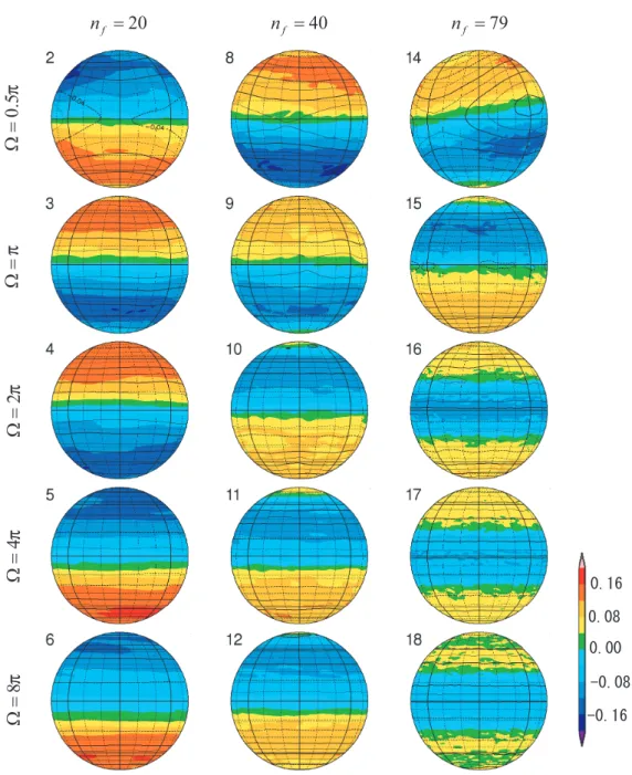
In all runs, the zonal flow structure becomes dominant from an early stage of time development. At around the time of the appearance of the zonal- band structure in Fig.2.3, the structure with alternating rather eastward and westward flows are already formed on a sphere (not shown). As time goes on, these flows become more zonal undergoing their mergers and disappearances, and fairly zonal flows have been formed by the final integration times in most of runs (Fig.2.8), though some large-scale and non-zonal equatorial flows, which are spoiling the zonal flows, are seen (runs 2,8,and 14), and there are several small non-zonal flows in the regions between the eastward and the westward flows (runs 15 and 16). The early emergence of the zonal- band structure and the realisation of the asymptotic with fewer zonal jets through the mergers and disappearances of the jets may tempt us to interpret the mergers and disappearances of the jets as a consequence of a barotropic instability of them. However, it should be remarked that, as pointed out by Rhines[4], a laminar zonal jet with a meridional scale larger than the Rhines scale is linearly stable owing to Rayleigh’s condition. Therefore, non-zonal flows superimposed on the zonal jets appear to be necessary for the merger and disappearance of the jets.

(34)

π5.0=Ωπ=Ωπ2=Ωπ4=Ωπ8=Ω

20

f =

n n_f =40 n_f =79

Figure 2.8: The stream function (contour lines) and zonal velocity (coloured) on a sphere at the ﬁnal integral time: t= 1×10⁵in runs 2−6,8,9,14,and 15, t = 1.2×10⁵ in run 10, t = 2.5×10⁵ in run 11, t = 1.6×10⁵ in run 12, t= 5.3×10⁵ in run 16,t = 5.2×10⁵ in run 17, andt = 5.7×10⁵ in run 18.

The top of the sphere, the bottom of the sphere, and the centre line in each panel correspond to the North Pole (90^◦ N), the South Pole (90^◦ S), and the equator, respectively. 32

(35)

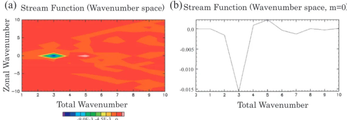
2.4 Stability of the 3-jet structure

-0.015 -0.010 0.0 -0.005

Stream Function (Wavenumber space) Stream Function (Wavenumber space, m=0)

Zonal Wavenumber

Total Wavenumber Total Wavenumber

-9.0E-3 -4.5E-3 0

(a) (b)

Figure 2.9: (a) The spectral distribution of the stream function ψ_n^m at t = 4.5×10⁵ in run 17 in the wavenumber space (For only 1 ≤ n ≤ 10,−10≤ m ≤10 is shown). The horizontal and the vertical axes are total wavenumber n and zonal wavenumber m in linear scale, respectively. (b) The spectral distribution of zonal component of the stream function ψ_n⁰ at t = 4.5×10⁵ in run 17 in the wavenumber space (For only 1 ≤ n ≤ 10 is shown). The horizontal and the vertical axes are total wavenumber n and the stream function ψ⁰_n in linear scale, respectively.

As we have seen in §2.3.1, the structure with three zonal jets seen in runs 16,17 and 18 is persistent and show little change for nearly 3×10⁵ of non-dimensional time, whereas the asymptotic states consist of two broad zonal jets in the rest of the runs. It is not clear if the broad 3-jet state is the asymptotic state of the system. Here we examine the robustness of 3-jet state in run 17 by adding small perturbations with (n, m) = (2,0) to the stream function, since the main component of the stream function of the 2-jet state in the wavenumber space is the one with n = 2, and observe whether the three jets experience a merger and disappearance to make 2-jets state or not.

Fig.2.9 shows the stream function at t = 4.5×10⁵ in run 17. Now let us magnify the (n, m) = (2,0) component of this stream function two, three, five, and ten times, then make temporal development taking each new flow as the starting flow field at t = 4.5×10⁵. The temporal variations of the zonal-mean zonal angular momentum [L_lon] fromt= 4.5×10⁵tot = 4.6×10⁵ are shown in Fig.2.10. In all cases, the three jets do not experience merger

(36)

and disappearance and are persistently remain until the final time. Further more, [L_lon] appears to go back to the 3-jet state even when the starting flow field consists of two strong jets and a very weak jet, the third (weakest) jet is enhanced in the course of temporal development, and the 3-jet state is reproduced at t = 4.6×10⁵. In fact, as shown in Fig.2.11, the absolute value of the (n, m) = (2,0) component of the stream function decreases, and the (n, m) = (4,0) component increases instead. This suggests that the 3-jet state in runs 16,17 and 18 are robust, and the structure with three broad zonal jets may be the long-time asymptotic state in these cases (runs 16,17 and 18).

34

(37)

Zonal-Mean Zonal Angular Momentum

LatitudeLatitude

0 90

-90 0 -90

90

4.5E5 4.6E5 4.5E5

4.5E5 4.5E5

4.6E5

4.6E5 4.6E5

Time Time

(a) (b)

(c) (d)

3

ψ

⁰₂

2

ψ

₂⁰

5

ψ

⁰₂

ψ

⁰₂10

0.036 −0.036

−0.072−0.036 0 −0.072 0 0.036

0.045

−0.072−0.036 0 0.036 −0.045

Zonal-Mean Zonal Angular Momentum Zonal-Mean Zonal Angular Momentum

Figure 2.10: Temporal development of zonal-mean zonal angular momentum [L_lon], started from a perturbed 3-jet state. The horizontal and the vertical axes in each panel are time and latitude in linear scale, respectively. The ﬂows are set to haveψ₂⁰ two (a), three (b), ﬁve (c), and ten (d) times as large as that in run 17 at t = 4.5×10⁵.