Weighted Least Squares with Orthonormal Polynomials and Numerical Integration for Estimation of Memoryless Nonlinearity
Kazuki Komatsu,Yuichi Miyaji,and Hideyuki Uehara,
Abstract—The nonlinearity of amplifiers is one of the major impairments in wireless communications. In this letter, we pro- pose a novel estimation method for the memoryless nonlinearity of amplifiers using weighted least squares and provide its theoretical error analysis on complex Gaussian signals. In the proposed method, the input signal and weight value are obtained via numerical integration formulas. Simulation results show that the proposed method can achieve a sufficiently low reconstruction error with 10 measurement samples on the estimation of the 13th- order nonlinearity. In addition, the simulation and theoretical results are consistent with each other.
Index Terms—Communication system nonlinearities, complex Gaussian process, least squares, nonlinear distortion, numerical integration
I. INTRODUCTION
WIRELESS communication systems suffer from the nonlinearities of amplifiers or other radio-frequency (RF) circuits. Accordingly, the estimation and compensation of these nonlinearities are important research objectives. The memoryless nonlinearity of an amplifier needs to be estimated accurately to achieve better pre-distortion [1] or better self- interference cancellation [2]. In the simplest model of the nonlinearity estimation problem, the relation between the input signalxn and the output signal yn can be written as
yn=f(xn) +zn, (1) where f(x) is the nonlinear transfer function of the target amplifier and zn is additive white Gaussian noise that is independent ofxnand distributed onCN(0, σ2z). In the model of (1), we focus on the accurate estimation of the transfer function of the amplifier with a small number of observation samples under the assumption that the output of the amplifier can be observed directly. The simplest solution of this problem is achieved using polynomial approximation and least squares estimation. Accordingly, the transfer function of the amplifier f(x)is approximated to the followingP-th order memoryless polynomial:
f(x)≈a1x+a3x|x|2+· · ·+aPx|x|P−1, (2)
This work was supported by the Japan Society for the Promotion of Science (JSPS) KAKENHI Grant Numbers JP18K04138, JP19K14979, and JP19J12727.
In this work, we used the cluster computer system of the Information Media Center (IMC), Toyohashi University of Technology.
The authors are with the Department of Electrical and Electronic In- formation Engineering, Toyohashi University of Technology, Japan (e-mail:
[email protected]; [email protected]; [email protected]).
and the coefficients a1, a3,· · · , aP are estimated using the following least squares method withN measurement samples:
ˆ a=
ˆ
a1 ˆa3 · · · ˆaPT
= XHX−1
XHy, (3) where (·)T and (·)H denote the transpose and Hermitian transpose of a matrix, respectively,ˆaprepresents the estimated coefficients, and
X=
x1 x1|x1|2 · · · x1|x1|P−1 x2 x2|x2|2 · · · x2|x2|P−1
... ... . .. ... xN xN|xN|2 · · · xN|xN|P−1
, (4)
y=
y1 y2 · · · yN
T
. (5)
However, this solution has severe numerical instability due to the large condition number of the Gram matrix XHX on high-order nonlinearity estimation [1], [3], [4]. Existing literature [1], [3], [4] provides an improved method for mit- igating the instability, using orthonormal polynomials instead ofx|x|p−1. Because of their advantages of orthonormality and orthogonality, orthogonal polynomials have been applied to not only estimation problems but also the latest studies on nonlinearities in a wide range of wireless communications such as the analysis of massive multiple-input multiple-output (MIMO) systems [5] and nonlinear equalizers [6].
In the improved version of the least squares estimation, the transfer functionf(x)is approximated to the followingP-th order expansion:
f(x)≈b1ψ1(x) +b3ψ3(x) +· · ·+bPψp(x), (6) whereψp(x)is ap-th order orthonormal polynomial. For the expansion (6), among the various types of orthogonal polyno- mials, a polynomial that satisfies the following orthonormality is used, to achieve better stability:
E
ψp(x)ψ∗q(x)
= Z
C
ψp(x)ψq∗(x)px(x)dx=δpq, (7) where δpq is the Kronecker delta, px(x) is the probability density function of x, and R
Cdxindicates integration on the complex plane. The orthonormal polynomial ψp(x) depends on the distribution of the communication signal because the expectation of (7) depends on it. Most current communica- tion systems use orthogonal frequency-division multiplexing (OFDM) as the modulation scheme. The complex amplitude of the OFDM signal is distributed on the complex Gaussian distribution due to a high number of subcarriers and the central
limit theorem [3], [7]. When the complex Gaussian signal has a unit variance, i.e., unit power, the orthonormal polynomial ψp(x), which satisfies the orthonormality of (7), can be written as
ψ2m+1(x) = (−1)m
√m+ 1L1m(|x|2)x, (8) where L1m(z) is the following generalized Laguerre polyno- mial:
Lαm(z) =
m
X
n=0
(−1)n n!
m+α m−n
zn. (9) Therefore, the estimated coefficient vector of the orthonormal expansion (6) obtained using the improved least squares can be expressed as
bˆ =ˆb1 ˆb3 · · · ˆbPT
= ΨHΨ−1
ΨHy, (10) where
Ψ=
ψ1(x1) ψ3(x1) · · · ψP(x1) ψ1(x2) ψ3(x2) · · · ψP(x2)
... ... . .. ... ψ1(xN) ψ3(xN) · · · ψP(xN)
. (11)
In (10), the (i, j)element of the Gram matrix ΨHΨ can be written as
ΨHΨ
i,j=
N
X
n=1
ψ∗2i−1(xn)ψ2j−1(xn). (12) When the number of measurementsNis sufficiently large, the equation
N→∞lim 1
N ΨHΨ
i,j=E
ψ2i−1∗ (x)ψ2j−1(x)
=δij (13) holds due to the orthonormality of ψp(x) because
1
N ΨHΨ
i,j is a sample average, and it converges to the expected value when N → ∞. Thus, (13) indicates that, if a sufficiently large number of measurement samples is available, the condition number of the Gram matrix converges to 1.
However, the convergence speed of (13) is very low when the measurement signal xn is randomly generated from a complex Gaussian distribution. The intuitive reason is that (12) is the Monte Carlo integration. It is known that the error of the Monte Carlo integration decreases as 1/√
N, and it is much slower than other numerical integration schemes. The same issue arises on ΨHy of (10). The i-th element of ΨHy is written as
ΨHy
i=
N
X
n=1
ψ2i−1∗ (xn)yn. (14) When the number of measurementsNis sufficiently large, the equation
N→∞lim 1
N ΨHy
i=E
ψ2i−1∗ (x)f(x)
= 1 π
Z
C
f(x)ψ2i−1∗ (x)e−|x|2dx=b2i−1 (15)
holds due to the orthonormality of ψp(x). However, the convergence speed of (15) is very low due to the Monte Carlo integration.
To summarize, the conventional least squares method has the following problems:
• Large condition number: When the number of measure- ment signals is not sufficient, the condition number of the Gram matrix becomes a large value.
• Low convergence speed: When the number of measure- ment signals is not sufficient, the estimated value does not converge to a true value.
These problems are related to random sampling observation, and the authors of the paper [8] proposed a sample selection method based on the genetic algorithm to solve these problems on digital pre-distortion with non-orthogonal polynomials. In contrast, in this letter, we propose a weighted least squares method with orthonormal polynomials and numerical integra- tion. In the proposed method, the measurement input signal xnand the weights of the least squares are easily obtained via numerical integration formulas.
The details of the proposed method are described in Sec- tion II. In Section III, the proposed scheme and the con- ventional least squares method are compared via numerical simulations. Section IV presents the conclusion of the letter.
II. PROPOSEDMETHOD
The proposed method uses the weighted least squares method. The measurement samples and weights are obtained using a numerical integration formula. In the proposed method, we approximate the transfer function to the orthonormal polynomial expansion of (6). Then, the vector of the estimated coefficients is expressed as
bˆ= ΨHWΨ−1
ΨHWy, (16) whereΨandyare the same as (11) and (5), respectively, and W = diag{w1, w2,· · ·, wN} is a diagonal weight matrix.
The main difference between the conventional and proposed methods is that the measurement samples xn and the weight wn are obtained using a numerical integration formula that can calculate the following two integrals:
E
ψ∗2i−1(x)ψ2j−1(x)
= 1 π
Z
C
ψ∗2i−1(x)ψ2j−1(x)e−|x|2dx, (17) E
f(x)ψ∗2i−1(x)
= 1 π
Z
C
f(x)ψ∗2i−1(x)e−|x|2dx, (18) with a high accuracy even if the number of measurementsN is very small. Generally, a numerical integration formula with N samples can be written as
E[g(x)]≈
N
X
n=1
g(xn)wn, (19) where g(x) is an arbitrary function, and xn and wn are the computing points and weights of the numerical integration, respectively. In the proposed method, we use the computing points as measurement samples, and then-th element of the
diagonal weight matrix W is wn. Then, we can expect that the following two equations:
ΨHWΨ
i,j =
N
X
n=1
ψ2i−1∗ (xn)ψ2j−1(xn)wn, (20)
ΨHWy
i=
N
X
n=1
ynψ2i−1∗ (xn)wn, (21) rapidly converge to the expected values of (17) and (18), re- spectively, if the noise is ignored. Therefore, the Gram matrix ΨHWΨbecomes the identity matrix, and the estimated vector bˆ stably converges to the true coefficient vectorb, even if the number of measurement samples is very small. In addition, if the Gram matrix is approximately the identity matrix, the estimate can be given asbˆ ≈ΨHWy.
A. Example 1: Gauss–Laguerre quadrature
The integrations of (17) and (18) can be rewritten as E[g(x)] = 1
π Z 2π
0
Z ∞ 0
g(rejθ)e−r2rdrdθ
= Z ∞
0
g(r)·2re−r2dr= Z ∞
0
g(√
t)e−tdt, (22) where g(x) = ψ2i−1(x)ψ2j−1∗ (x) for (17), and g(x) = f(x)ψ2i−1∗ (x) for (18). The reason for the above transfor- mation is that g(x) = g(|x|) holds in both cases. The last term of (22) is a semi-infinite integral with an exponentially decaying weight function, and the Gauss–Laguerre quadrature is a good choice for integrating it with high accuracy. In the Gauss–Laguerre quadrature, the computing pointtn is then- th root of the Laguerre polynomial LN(x) =L0N(x), and the weights are given by [9, Eq. 25.4.45]
wn0 = xn
(N+ 1)2[LN+1(xn)]2. (23) Then, the measurement samples and weights of the proposed method are xn=√
tn andwn=w0n, respectively. Moreover, the error of the Gauss–Laguerre quadrature is given by [9, Eq.
25.4.45]
RN[g] = (N!)2 (2N)!
d2N dt2Ng(√
t) t=ξ
. (0< ξ <∞) (24) Thus, the convergence speed of the Gauss–Laguerre quadra- ture is much higher than that of the Monte Carlo integration because (N(2N!))!2 2−N.
In Section III, when the number of measurements is larger than 100, the 100 measurement samples and weights are repeated N/100 times to generate N measurement samples and weights because the Gauss–Laguerre quadrature has very high accuracy, even ifN= 20. Thus, we usexn =pt(n%100) and wn = 100N w0(n%100) when N > 100, where the binary operator% indicates the remainder after division, and tn and wn are obtained from 100-points Gauss–Laguerre quadrature.
B. Example 2: Rectangular rule
Generally, the rectangular rule is not a highly accurate integration method, but it is practical for the proposed method.
The middle term of (22) is an integration with a rapidly decreasing weighte−r2, and we can obtain sufficient accuracy even if the integration interval is only[0,5]instead of[0,∞).
Then, the measurement samples and weights of the proposed method with the rectangular rule can be written as
xn = 5
Nn, wn =10
Nxne−x2n. (25) In (22), the integrand can be approximated to zero at both ends of the integration domain, i.e.,g(r)·2re−r2 ≈0atr= 0and r= 5. Then, the rectangular rule for (22) is almost equal to the trapezoidal rule, and the error of the integration can be expressed as [9, Eq. 25.4.2]
RN[g]≈ 125 12N2
d2 dr2
h
g(r)·2re−r2i r=ξ
.(0< ξ <5) (26) Thus, the convergence speed of the rectangular rule is higher than that of the Monte Carlo integration because RN[g] ∼ O(N−2).
It can be observed from (25) that the measurement samples can be viewed as a ramp signal. This is an interesting aspect of the rectangular rule for the proposed method.
C. Theoretical error analysis
In this subsection, we analyze the following total recon- struction error:
Etot2 =E
f(x)−fˆ(x)
2
, (27)
wherefˆ(x)is the reconstructed nonlinearity defined as fˆ(x) = ˆb1ψ1(x) + ˆb3ψ3(x) +· · ·+ ˆbPψP(x). (28) Furthermore, the nonlinear functionf(x)can be expanded to an infinite series as
f(x) =b1ψ1(x) +b3ψ3(x) +· · ·=
∞
X
p=1,3,···
bpψp(x). (29) Thus, the total error can be rewritten as
Etot2 =E
P
X
p=1,3,···
(bp−ˆbp)ψp(x) +
∞
X
p=P+2,P+4,···
bpψp(x)
2
(a)=
P
X
p=1,3,···
E
bp−ˆbp
2
| {z }
Estimation error:Eest2
+
∞
X
p=P+2,P+4,···
|bp|2
| {z }
Approximation error:Eapp2
. (30)
The transform of(a)= is due to the orthonormality of (7). The proposed method has two errors: the estimation errorEest2 and the approximation errorEapp2 . The approximation error is the error caused by approximating the series expansion off(x)in finite dimensions. The conventional method also has this error
due to the approximation of (6). The approximation error can be written as [10, eq. (3.2.7), section 3.2, p. 217]
Eapp2 =E
|f(x)|2
−
P
X
p=1,3,···
E
f(x)ψp∗(x)
2. (31) In (31), the approximation error monotonically decreases as the order P increases. This error has the same value in both the proposed and conventional methods if the order P is the same.
In contrast, the estimation errorEest2 leads to a performance variation between the proposed and conventional methods.
When the Gram matrix converges to the identity matrix sufficiently, the estimated coefficientˆbp can be written as
ˆb2i−1= ΨHWy
i
=
N
X
n=1
f(xn)ψ∗2i−1(xn)wn+
N
X
n=1
znψ2i−1∗ (xn)wn. (32) Thus, the estimation error E2estcan be rewritten as
Eest2 =
P
X
p=1,3,···
N
X
n=1
f(xn)ψp∗(xn)wn−bp
2
+
P
X
p=1,3,···
E
N
X
n=1
znψ∗p(xn)wn
2
. (33) In the right-hand side of (33), the first term indicates the square of the quadrature error, and the second term indicates the error caused by the noise. The square of the quadrature error is RN[f(r)ψ∗p(r)]2
, and the error rapidly decays at a rate ofO(N−4), even for the rectangular rule. In addition, the noise error can be rewritten as
P
X
p=1,3,···
E
N
X
n=1
znψ2i−1∗ (xn)wn
2
=σ2z
P
X
p=1,3,···
N
X
n=1
|ψp(xn)wn|2. (34) Equation (34) shows that the effect of noise depends on the values of the measurement samples and weights determined by the numerical integration method employed, and the sum of their squares is an indicator of the influence of noise. When the rectangular rule is used for the proposed method, the summation of the right-hand side of (34) with a largeN can be asymptotically expressed as
N
X
n=1
|ψp(xn)wn|2≈ 5 N
Z ∞ 0
n
ψp(xn)·2re−r2o2
dr∼ O(N−1).
(35) The noise error decays at a rate ofO(N−1), and the quadrature error is negligibly small compared with the noise error.
To summarize this section, we can estimate the error of the proposed method as
E2tot≈E2app+σz2
P
X
p=1,3,···
N
X
n=1
|ψp(xn)wn|2. (36) The first term is a constant for the number of measurements N, and the second term decays at a rate ofO(N−1). Thus, the
101 102 103 104 105
The number of measurements:N 100
101 102 103 104 105 106 107
ConditionnumberofGrammatrix
Ga.Lag.
Rect.
Conv.
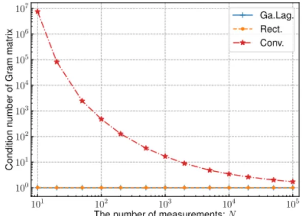
Fig. 1. Condition number of the Gram matrix of each method whenP = 7.
The value is averaged over104 times independent Monte Carlo simulation.
convergence rate of the proposed method is the same as that of the conventional Monte-Carlo-based least squares method whose rate of square error is O(N−1). This is because the conventional method is exactly same as the proposed method with randomly generated samplesxnand weightswn= 1/N.
However, the rate is a characteristic of N → ∞, and we compare the characteristics of each method from a small to a large numberN in numerical experiments in the following section.
III. RESULTS OFNUMERICALEXPERIMENTS
In this section, we evaluate and compare the condition number and total reconstruction error, which is defined as (27), for the proposed and conventional methods using 104 times Monte Carlo simulation. In the simulation, we use the Rapp model [11] as an amplifier, and its transfer function can be written as
f(x) = x
1 + (|x|/B)2s2s1
, (37)
where B indicates the input back-off (IBO), and s is the smoothness factor. Furthermore, we useB=√
10(i.e., 10 dB IBO) ands= 3.
Figure 1 shows the condition number of the Gram ma- trix of each method. As mentioned in the Introduction, the condition number of the conventional method is much larger than that of the proposed method because it is based on the Monte Carlo integration. The proposed method successfully reduces the condition number because of its high accuracy of numerical integration. This indicates that the proposed method can achieve better stability than the conventional least squares method.
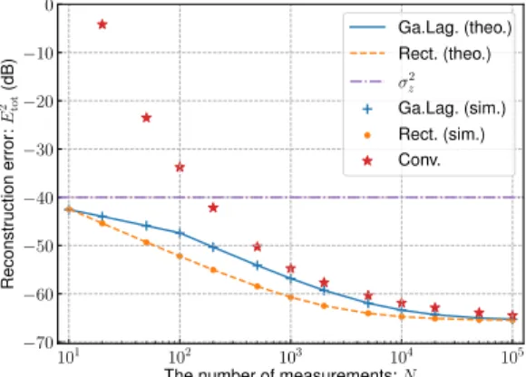
Figures 2, 3, 4, and 5 show the simulation results and theoretical results of the total reconstruction error for each method, withP = 7andP = 13, from a very noisy case to an almost noise-free case for a wide range of applications such as pre-distortion, post-distortion, and self-interference cancellers.
The error of the proposed method is much smaller than that of the conventional method, as the proposed method has good stability and better accuracy of integration. Surprisingly, even when only 10 measurements are used, the proposed method maintained the reconstruction error below the noise.
101 102 103 104 105 The number of measurements:N
−30
−20
−10 0 10 20
Reconstructionerror:E2 tot(dB)
Ga.Lag. (theo.) Rect. (theo.) σ2z
Ga.Lag. (sim.) Rect. (sim.) Conv.
Fig. 2. Total reconstruction error Etot2 of each method with P = 7 and σ2z = 101. The lines indicate theoretical results, and the markers indicate simulation results.
101 102 103 104 105
The number of measurements:N
−50
−40
−30
−20
−10 0
Reconstructionerror:E2 tot(dB)
Ga.Lag. (theo.) Rect. (theo.) σ2z
Ga.Lag. (sim.) Rect. (sim.) Conv.
Fig. 3. Total reconstruction errorEtot2 of each method withP = 13and σ2z = 10−1. The lines indicate theoretical results, and the markers indicate simulation results.
101 102 103 104 105
The number of measurements:N
−70
−60
−50
−40
−30
−20
−10 0
Reconstructionerror:E2 tot(dB)
Ga.Lag. (theo.) Rect. (theo.) σ2z
Ga.Lag. (sim.) Rect. (sim.) Conv.
Fig. 4. Total reconstruction error Etot2 of each method with P = 7 and σ2z = 10−4. The lines indicate theoretical results, and the markers indicate simulation results.
In contrast, in Fig. 2, the error of the conventional method is smaller than that of the proposed method when N > 104. Therefore, the conventional method is more effective than the proposed method when a sufficient number of samples are used under low signal-to-noise ratio (SNR). In addition, the theoretical and simulation results are consistent with each other in these figures. Thus, the analysis in this paper is useful for the error estimation of the proposed method. Moreover, if the error is to be reduced further, a numerical integration method that reduces the value of (34) needs to be used.
101 102 103 104 105
The number of measurements:N
−80
−60
−40
−20 0
Reconstructionerror:E2 tot(dB)
Ga.Lag. (theo.) Rect. (theo.) σz2
Ga.Lag. (sim.) Rect. (sim.) Conv.
Fig. 5. Total reconstruction errorEtot2 of each method withP = 13and σz2= 10−7. The lines indicate theoretical results, and the markers indicate simulation results.
IV. CONCLUSION
In this letter, we proposed a novel estimation method for the memoryless nonlinearity of an amplifier. The method uses weighted least squares with orthonormal polynomials and numerical integration. The measurement signal and weights of the proposed method were designed based on the numerical integration method to converge the Gram matrix to the unit matrix with high accuracy, even with a small number of observations. Moreover, we derived the theoretical error of the proposed method. The simulation results showed that the proposed method dramatically improved the accuracy of the conventional least squares method and achieved sufficient accuracy with 10 measurement samples. The theoretical results and simulation results were consistent with each other.
REFERENCES
[1] H. Qian, S. Yao, H. Huang, and W. Feng, “A low-complexity digital predistortion algorithm for power amplifier linearization,”IEEE Trans.
Broadcast., vol. 60, no. 4, pp. 670–678, Dec. 2014.
[2] K. Komatsu, Y. Miyaji, and H. Uehara, “Basis function selection of frequency-domain Hammerstein self-interference canceller for in-band full-duplex wireless communications,”IEEE Trans. Wireless Commun., vol. 17, no. 6, pp. 3768–3780, Jun. 2018.
[3] R. Raich and G. Zhou, “Orthogonal polynomials for complex Gaussian processes,”IEEE Trans. Signal Process., vol. 52, no. 10, pp. 2788–2797, Oct. 2004.
[4] R. Dallinger, H. Ruotsalainen, R. Wichman, and M. Rupp, “Adaptive pre-distortion techniques based on orthogonal polynomials,” in Proc.
44th Asilomar Conf. Signals, Syst., Comput., Nov. 2010, pp. 1945–1950.
[5] S. Teodoro, A. Silva, R. Dinis, F. M. Barradas, P. M. Cabral, and A. Gameiro, “Theoretical analysis of nonlinear amplification effects in massive MIMO systems,” IEEE Access, vol. 7, pp. 172 277–172 289, 2019.
[6] L. Shen, B. Henson, Y. Zakharov, and P. D. Mitchell, “Adaptive nonlinear equalizer for full-duplex underwater acoustic systems,”IEEE Access, 2020, (Early Access, DOI:10.1109/ACCESS.2020.3000590).
[7] P. Banelli and S. Cacopardi, “Theoretical analysis and performance of OFDM signals in nonlinear AWGN channels,”IEEE Trans. Commun., vol. 48, no. 3, pp. 430–441, Mar. 2000.
[8] J. Kral, T. Gotthans, R. Marsalek, M. Harvanek, and M. Rupp, “On feed- back sample selection methods allowing lightweight digital predistorter adaptation,”IEEE Trans. Circuits Syst. I, vol. 67, no. 6, pp. 1976–1988, 2020.
[9] M. Abramowitz and I. A. Stegun,Handbook of Mathematical Functions with Formulas, Graphs, and Mathematical Tables. New York City:
Dover, 1964.
[10] W. Gautschi, Orthogonal Polynomials: Computation and Approxima- tion, ser. Numerical mathematics and scientific computation. Oxford University Press, 2004.
[11] C. Rapp, “Effects of HPA-nonlinearity on a 4-DPSK/OFDM-signal for a digital sound broadcasting system,” inProc. the Second Europian Conf.
on Satellite Commun., Oct. 1991, pp. 179–184.