BREAK‑EVEN ANALYSIS AND FIXED OVERHEAD COSTING
著者 Suemasa Yoshinobu
journal or
publication title
關西大學商學論集
volume 11
number 2
page range A222‑A179
year 1966‑06‑27
URL http://hdl.handle.net/10112/00021529
BREAK-EVEN ANALYSIS AND FIXED OVERHEAD COSTING*
By
Y oshinobu Suemasa
CONTENTS I Introduction
II Basic Relationships
III Break-even Analysis in Actual Absorption Costing IV Break-even Analysis in Standard Absorption Costing
V Mechanism of Break-even Analysis in the Theoretical Calculation VI Occasional Break-even Analysis in Standard Absorption Costing VII Break-even Analysis in Absorption Costing for Interim Reports VIII Break-even Analysis in Direct Costing
IX Some Conditions for Planning Purpose
X Consideration of a Certain Profit or Maximum Profit XI Summary and Conclusions
I INTRODUCTION
222
In profit planning or profit forecasting, break-even analysis is an essential tool. There are several assumptions in conventional break-even analysis.
For example:
( 1 ) Costs can be partitioned into their fixed and variable components.
( 2 ) Price of the product does not change.
* This paper should not be quoted or reproduced in whole or in part without the consent of the author.
I express my gratitude to Professor Oswald Nielsen of Stanford University, for he has provided me with opportunities for accounting study at Stanford University, as well as detailed review and helpful· suggestions. I wish also to acknowledge detailed review and helpful suggestions from Yuji Ijiri of Stanford University and Arne Kinserdal of Norges Handelshcpyskole, Bergen.
( 1 )
( 3 ) Only one product is involved, or sales mix and product mix remain constant.
( 4 ) Production volume and sales volume are always equal.
Conventional break-even analysis has some weak points. Professor Nicker- son points out one weak point as follows: "A major weakness of a break-even chart as a check up device, however, is that the assumption has been made that sales volume and production_ volume are identical, ... this is not likely to be the case."1
In most companies, production volume and sales volume are not always equal for short-run periods, and beginning inventories and ending inventories are different both in the unit price and in the volume. Therefore, the income statement and profit budget plan depend upon their methods of cost accounting and inventory valuation. That is, they depend upon the method of charging fixed overhead costs to inventories. Then the mechanism of profit planning should be harmonized with the mechanism of profit reporting by income statement.2 In this case, the break-even analysis must treat profit and volume relations under the assumption that production volume and sales volume differ.
Such a break-even analysis will be of more use for profit planning and control, especially budgetary control, than the conventional break-even analysis. I want to discuss break-even analyses under some methods of-cost accounting.
More specifically, I would like to discuss the break-even analysis under the following assumptions:
( 1 ) Costs can be partitioned into fixed and variable components.
(2) ( 3) . ( 4)
Price of the product does not change.
Only one product is produced and sold.
Unit variable costs and absorbed fixed costs per unit (unit fixed cost portion) in beginning inventories are equal to that of production costs in the current period. This simplification is assumed so that the calculations by every method of inventory costing (e.g. average cost,
1. Clarence B. Nickerson, Managerial Cost Accounting and Analysis: Text, Problems and Cases (New York: McGraw-Hill Book Co., 1962), p. 387.
2. R. Lee Brummet, Overhead Costing: The Costing qf Maunfactured Prodw;ts (Ann Arbor: Bureau of Business Research; School of Business Administration, University of Michigan, 1957), p. 100.
BREAK-EVEN ANALYSIS AND FIXED OVERHEAD COSTING (Suemasa) 220 Fifo, Lifo, etc.) result in the same effect.
( 5) Budgeted (standard) cost figures and actual cost figures are identical.
This simplification is assumed so that under-or over-absorbed manufactur- ing overhead cost is composed on only volume variance ( or capacity variance).
The above-mentioned assumptions are mainly for planning purposes.
However, for control purposes, assumptions (4) and (5) may be appropriate.
Therefore, in my next paper, I want to approach break-even analysis techniques which do not follow the above-mentioned .assumptions.
References
I. Kazuto Kunihiro, Break-Even Anarysis (Tokyo: Chuokeizaisha, 1952).
2. Gibert Amerman, "Facts About Direct Costing for Profit Determination,"
· Accounting Research, Vol. V, No. 2 (April, 1954).
3. Clarance L. Van Sickle, Cases in Cost Accounting (Englewood Cliffs, N. J.: Pren- tice-Hall, Inc., 1955).
4. Kazuto Kunihiro, Practical Financial Statement Anarysis (Tokyo: Daiyamondosha, 1956).
5. R. Lee Brummet, Overhead Costing: The Costing of Manufactured Products (Ann Arbor: Bureau of Business Research, School of Business Administration, The Uni- versity of Michigan, 1957).
6. Glenn A. Welsch; Budgeting:. Profit Planning and Control (Englewood Cliffs, N. J.:
Prentice-Hall, Inc., 1957 and 2d ed. 1964).
7. Takeo Takemitsu, "On the Seeking Methods of Break-Even Analysis Where Production Volume is Unequal to Sales Volume", Sangyokeiri, Vol. XXVII, No.
6. (June, 1957.)
8. Kazuto Kunihiro, "Problem and Modernization of Profit Planning," Kigyokaikei, Vol. XIX, No. II (October, 1957.)
9. Otojiro Kubota, "On the Relationships of Profit Planning and Cost Accounting,"
Kigyokaikei, Vol. XX, No. 6 (June, 1958.)
10. Albert W. Patrick, "Some Observations on the Break-Even Chart", Accounting Review, Vol. XXIX, No. 4 (October, 1958).
11. Roy E. Tuttle, "The Effect of Iq.ventory Change on Break-Even Analysis,"
N. A. A. Bulletin, Vol. XL, No. 5 (January, 1959).
12. Wilbert C. Wehn, "Points That Mean More in Profit Control", The Controller, Vol. XXVII, No. 7 (July, 1959).
13. Yoshinobu Suemasa, "Profit Planning and Break-Even Analysis", Kansai Univer- siry Keizai-Seiji Kenkyusosho, No. 2 (October, 1959).
14. William]. Vatter, "Toward a Generalized Break-Even Formula", N.A.A. Bulleti[,, Vol. XLIII, No .. 4- (December, 1961).
15. Porter W. Henderson and Horace R. Brock, "Imbalanced Volume Breakeven Analysis for Use With the Comprehensive Budget Program'', Budgeting, Vol. XIII, No. 2 (November, 1964-).
16. William A. Terrill and Albert W. Patrick, Cost Accounting For Management (New York: Holt, Rinehart and Winston, Inc., 1965).
II BASIC RELATIONSHIPS
Break-even analysis should be treated under the conditions of the following basic relationships.
(I) Types of costing systems.
The types of costing systems are divided into four groups. For example, Professor Horngren has summarized them as follows: 1
I. Actual-Normal Absorption Costing.
2. Actual-Nornial Direct Costing.
3. Standard Direct Costing.
4. Standard Absorption Costing.
Variable overhead costs are predetermined under the above four costing systems and are included in the product cost. Fixed overhead costs are predetermined under absorption costing and are included in the product cost. Needless to say, predetermined costs under actual absorption costing differ with predetermined costs under standard absorption costing. Namely, these costs under actual costing are estimated costs, but these costs under standard costing are standard or budgeted costs. Therefore, the nature and disposition of the cost variances depend upon the nature of predetermined costs under each costing. Especially, it seems that the effect of the charge methods for fixed costs is very important for profit planning or profit for_ecasting.
In this paper, I will make the following assumptions. The predetermined unit variable overhead cost and the predetermined total fixed overhead cost
1. Charles T. Homgren, Accounting For Management Control: An Introduction (Engle- wood Cliffs, N. J.: Prentice-Hall, Inc., 1965), p. 4-10.
BREAK-EVEN ANALYSIS AND FIXED OVERHEAD COSTING (Suemasa) 218
are the same under each costing system. But, the effect of the charge for fixed overhead costs differ among actual absorption costing and. standard absorption costing and direct costing. Actual and standard direct. costing coincide with respect to disposing of fixed overhead cost. Accordingly, I intend to approach each break-even analysis under (1) actual absorption costing ( complete actual absorption costing and actual-normal absorption costing), (2) standard absorption costing, and (3) direct costing.
(II) Disposing of fixed overhead cost variance.
Fixed overhead cost variances are caused by using the fixed overhead burden rate under absorption costing, but their variances do not occur under direct costing. The fixed overhead cost variances are disposed of by various methods. These methods could be summarized as follows:
A. Distribution to the inventories and cost of goods sold.
1. The variance is charged to each production order account by a sup- plemental burden rate at the end of the month or the costing period.
2. The variance is prorated over the inventories (work in process and finished goods) and cost of goods sold at the end of the month or the accounting period.
B. Charge to period costs.
1. The total variance accrued in the period is charged to the cost of goods sold account at the end of the month or the accounting period.
2. The total variance accrued in the period is charged to non-operating expense or income account at the end of the month or the accounting period.
C. Charge as period costs within the range of a certain limited amount, and distribution to the inventories and cost of goods sold without the range of a certain limited amount.
1. The variance accrued in the period is charged to the non-operating expense account within the range of a certain limited amount at the end of the month or the accounting period.
2. The variance accrued in the period is prorated over the inventories and cost of goods sold without the range of a certain limited amount at the end of the month or the accounting period.
D. Carry forward to the coming period.
( 5 )
I. The variance is shown on the interim balance sheets as either a deferred charge or a deferred_ credit at:the end of the month.8 2. The variance is shown on the periodic balance sheet as either a
deferred charge or a deferred credit at the end of the accounting period.
The selection of the disposing method is connected with the nature of the accounting report of each period and the type of costing system. For example, in the interim report, the disposing method frequently selects the D method of carrying forward to the coming period. But the D method of carrying forward to the coming period is rarely selected on the accounting periodic report. Then in actual absorption costing, the disposing method frequently selects A method of distributing to the inventories and cost of goods sold.
And in the standard absorption costing, B method of charging to the period cost is almost always selected as the disposing method.
My standpoint attaches importance to the clearness of profit reckoning and profit budget plan. Therefore, I intend to readjust as follows:
( 1 ) The fixed overhead cost variance in actual absorption costing may be disposed by the A method of distributing to the inventories and cost of goods sold.
( 2 ) The cost variance in standard absorption costing may be disposed by the B method of charging to the period cost.
( 3 ) On the oc~asion that the cost variance disposing method is compelled by requisition of the external financial report and/or· income tax report, the cost variance in standard costing may be disposed by the C method.
( 4 ) There are many cases where disposing the variance for the interim report is distinguished from the above three readjustments. On that occasion, the cost variance in the actual absorption costing and standard absorption costing is disposed by the D method of carrying forward to the coming period.
Accordingly, in absorption costing, I intend to treat each break-even analysis under the above-mentioned four readjustments.
(III) The following notations are used in every break-even analysis.
F 1 = Fixed manufacturing costs.
2. · William J. Vatter, "Toward a Generalized Break-Even Formula," N. A. A.
Bulletin, Vol. XLIII, No. 4 (December, 1961), pp. 6-10.
BREAK-EVEN ANALYSIS AND . FIXED OVERHEAD. COSTING (Suemasa) 216
V 1 = Variable manufacturing costs. The same per unit= v1
F2=Fixed selling and administrative costs
V2= Variable selling and administrative costs. The same per unit=v2
· S=Sales in budgeted income statement. The same per unit=s BE= Break-even sales
x=Predetermined sales volume in budgeted income statement.
x" = Break-even sales volume
y=Predetermined production volume in budgeted income statement.
y"=Estimated production volume with a view to determine fixed over- head burden rate in actual costing.
y*=Standard (or budgeted) production volume with a view to determine fixed overhead burden rate in standard costing.
And then, S=sx, BE=sx".
(IV) The fact that conventional break-even analysis assumes that production volume and sales volume are equal can be expressed as follows:
Conventional break-even formula:
BE F1+F2
V1+V2
s
F1+F2
The following income statements are used as simplified data.
Budgeted Income Statements Item
Sales
Cost of goods sold
Case I y=60,000
x=60,000 600,000 Beginning inventory 0
Production cost
Fixed costs 200,000 Variable costs 210,000
Case II y=80,000 x=60,000 600,000 0
200,000 280,000
Case Ill y=lOO~OOO
X= 60,000 600,000 0
200,000 350,000
Cost of goods avail-
able for sales 410,000 480,000 650,000
Ending inventory 0 410,000 120,000 360,000 220,000 330,000
Gross margin 190,000 240,000 270,000.
Selling and adminis- trative costs
Fixed costs 100,000 100,000 100,000
Variable costs 90,000 190,000 90,000 190,000 90,000 190,000
Net income 0 50,000 80,000
The basic figures of Case I in the above income statements are given in the following table:
F 1 = ¥200,000 V 1 = ¥210,000 F 2=¥100,000 V2=¥90,000 S=¥600,000
[email protected] S=@ ¥10.00
And the previous formula can be reckoned as follows:
Conventional formula
BE 200,000+ 100,000 l 210,000+90,000
600,000 BE 200,000+ 100,000
l 3.5+1.5 10
=600,000
The conventional break-even sales point of ¥600,000 coincides with zero profft sales in the Case I. Namely, under the y=60,000 and x=60,000, the effect of the break-even sales computations coincides with Case I in the income statements. However, in Case II and III, although both sales of the
¥600,000 are equal to the break-even sales of ¥600,000, profits are not zero, but ¥50,000 in Case II and ¥80,000 in Case III.
Supposing the fundamental device of the conventional break-even formula is used, break-even analysis needs to be reconsidered under the mechanism of each costing system, taking into consideration the four basic relations.
( 8 )
BREAK-EVEN ANALYSIS AND FIXED OVERHEAD COSTING (Suemasa) 214
m BREAK-EVEN ANALYSIS IN ACTUAL ABSORPTION COSTING Break even analysis in complete actual absorption costing typically is divided into three types which are described as follows. Their formulas depend upon the assumption of y=f• in conclusion.
A. The cost of goods sold is calculated as a numerator in the break-even formula.1
Cost of goods sold=(F1+ V1) -y X
CF1+V1)-+F2 y X
BE
Fi-=-+ Vc=-+F2
- ~ y - ~ y ~ - ... (}) 1 - ~
s
B. The fixed cost component in the cost of goods sold is calculated as a numerator in the break-even formula.9 Namely, [Fixed manufacturing cost - Inventoried fixed cost] is calculated as a numerator in this formula.
Fixed cost components in the cost of goods sold=F1---=---y
F1-+F2 X
BE y
v1---=---+v2
1- y
sx
···(2)
C. The cost of goods sold is not calculated as a numerator, but is calcula- ted as a portion of the denominator in the break-even formula. 3 I. Kazuto Kunihiro, Practical Financial Statement Anav,sis (Tokyo: Daiyamondosha,
1951), pp. 63-65.
2. Glenn A. Welsch, Budgeting: Profit Planning and Control (Englewood Cliffs, N. J.:
Prentice-Hall, Inc., 2d ed. 1964), pp. 343-345.
3. Yoshinobu Suemasa, "Profit Planning and Break-Even Analysis", Kansai Uni- versi!)I Keizai-Seiji Kenkyusos/w, No. 2 (October, 1959).
BREAK-EVEN ANALYSIS AND FIXED OVERHEAD COSTING (Suemasa)
s
_ _ _ F___,F~1--- ... (3) v1+--+v2 y
s
The following figures are given in the formulas.
F1=¥200,000 V1=@¥3.50
V2=@¥1.50 s=@¥10.00
Each formula can be calculated as follows:
A method.
BE 200,000~+ 3.5x+ 100,000 y
1 _ ____!_2_
10
200,000~+3.5x+ 100,000
- - ~ y " ---,---- ... (1') 0.85
B method.
BE
200,000~+ 100,000 y
1-10 5
200,000~+ 100,000
- - ~ y " - - - - ... (2') 0.5
C method.
BE
1
100,000 3.5+ 200,000 + 1.5
y
_ _ 1~00---',,,o~o~o _ _ ... (3') 200,000 +5
y 10
Under a given y (predetermined production volume in budgeted income
BREAK-EVEN ANALYSIS AND FIXED OVERHEAD COSTil'TG (Sueniasa) 212
statement) in every formula, break-even sales cannot be determined in formulas ( 1 ') and (2'), unless x (predetermined sales volume in budgeted income statement) is given. That is, the break-even sales point under formulas (1') and (2') can be determined under a givetiy and x. But the purpose ofbreak- even analysis for profit planning is to seek possible break-even sales or goal sales which include a certain profit under some given conditions. Therefore, it seems that a given x (predetermined sales volume) should not be given previously in the break-even sales calculation. Formulas (l') and (2') cannot solve the problem ,unless x is given.
Tentatively, if x (predetermined sales volume) is given various values, break- even sales are determined by formulas (1'), (2') and (3') as follows:
Under the condition of y= 100,000 Formula
Formula Formula
(l ') (2') (3')
x=I00.000
¥764.604
¥600.000
¥333.333
x=50.000
¥441.176
¥400.000
¥333.333
x=33.333
¥333.333
¥333.333
¥333.333
'l;'herefore, the A method of formula ( l ') and the B method of formula (2') have discrepant break-even sales in each given predetermined sales volume (x) under a given predetermined production volume (y)4 • Accordingly, I think that the C method. of (3') is valuable and useful in break-even analysis under actual absorption costing.
4. If the break-even sales lines are plotted by break-even formula (2'), break-even sales lines could be drawn as follows:
100.000 units
A s
L E s
Diagram III
x=l00.000 units x= 75.000 units x= 50.000 units x= 33.333 units bold line is drawn by the C method 0 .__ _ _ P_R_O __ D,..,U'"'c-=T::::I-=o-:-cN,---1-0-0.000 units
The validity of computation by C method of formula (3') may be verified as follows:
Income Statement Break-even sales (x=33.333)
Cost of goods s~ld
Production cost (y= 100.000) Fixed costs
Variable costs
Total production costs Less inventory (66.667 units) Gross margin
Selling and admininistrative costs Fixed costs
Variable costs Net income
333.333
200.000 350.000 550.000
366.667 183.333 150.000 100.000
50.000 150.000 Nil The calculation by formula (3') coincides with the income statement above.
Therefore, the calculations by formulas (l') and (2') seem to be misleading.
Moreover, under the condition of y ~ yt>. (predetermin.ed production volume in budgeted income statement ~ estimated production volume used for fixed overhead burden rate) in actual-normal absorption costing, under- or over- absorbed fixed cost is often distributed to inventories and cost of goods sold in actual absorption costing. C method of formula (3) is described as follows:
Estimated fixed cost component in cost of goods sold
y X
=F1X - - X - yt>. y
X
=F1 yt>.
Under- or over-absorbed fixed cost to be distributed to cost of goods sold
BE X X X
v1x+ F 1y+ v2x+ F 1y - F 1y
sx
···•(4)
BREAK-EVEN ANALYSIS AND FIXED OVERHEAD COSTING (Suemasa) 210
s
Consequently, the final formula derived by formula (4) coincides with formula (3). For that reason, it seems that break-even analysis in actual absorption costing may be of great use in formulas (3) and (3') from the first calculation.
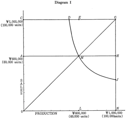
Further if various production volumes are given in place of JI in the formula (3'), each break-even sales on various production volumes can be easily de- termined. And each break-even sales can be plotted as a break-even sales line in the following diagram I. Subsequently, the break-even sales line is depicted as the DMJ curve line in the diagram.
5. Professor Welsch assumes "that the percentage inventory increase or decrease will tend to be proportional to charges in production", (op. cit., p. 343). His break- even sales formula is based on this assumption. But it seems that this assumption is not necessary in break-even analysis. My exercise may be verified by his ver- ification method (op. cit., p. 344) as follows:
Income Statement Break-even sales .(40.000 units)
Cost of goods sold
Production cost (40.000+0.50=80.000) Fixed costs
Variable costs Total production costs
Less inventory (50% of production) Cost of goods sold
Gross margin
Selling and administrative costs Fixed costs
Variable costs Net income
400.000
200.000 280.000 480.000 240.000
240.000 160.000 100.000
~ 160.000
N i l
But my exercise uses 100.000 units of production volume (y) in. the income state- ment. His verification method differs from the income statement because of his assumption. Therefore, I could not use his break-even calculation formula.
( 13 )
Diagram I
C.,__ _ _ _ _ _ _ _ _ _ D _ _ E _ _ _ _ _ _ _ ...,.G
¥1,000,000 (100.000 units)
A s
L E s
J
L N
0 ---P-R-O~D_U_C_T.._IO_N_~--¥-60 .... 0-,0-00~--'---=¥-=-1-,o:-::o~o.-=-oo:-::o:-- ( 60.000 units) (100. 00Ounits) Therefore, an essential problem lies in the fact that x is used as a known number. Essentially, break-even analysis seeks possible break-even sales or goal sales. Accordingly, the inventories in break-even formulas should be cal- culated as follows:
Predetermined inventories volume increase or decrease
Predetermined production volume
Break-even sales vol- ume or goal sales vol- ume calculated in the break-even formula Then, the cost of goods sold in break-even formulas should not be equivalent to predetermined sales, but should correspond with the break-even sales.
Therefore, x should not be treated as a known number, but rather an unknown number x". The undecided x" can be used in place of a given x, because in each unit v1, v2 and s, it is used as a variable of the sales volume, and F 1~
y
BREAK-EVEN ANALYSIS AND FIXED OVERHEAD COSTING (Suemasa) 208 (fixed costs in predetermined cost of goods sold), Ve~ (variable costs in pre-
y
determined cost of goods sold) and (F1+ V1)2'... (predetermined cost of goods y
sold) are used equally, as a variable of the sales volume under a given y. Then, an x11 should be shifted to the x places. Needless to say, x11 has not changed the nature of the sales function like x did. Thus, the previously mentioned formulas (1), (1'), (2), (2'), (3) and (3') are revised as follows:
By the formula ( 1) x"
(F1+ V1) - + F2
s x "=----~Y~-- I - ~
... (RI)
s
By the formula ( l ')
200.000,-~-=-+3.5x11+ 100.000 IOx11 y
0.85
8.5x 11 = 200.000...:..:_+ 3.5x 11 + I 00.000 y
... (RI')
5x11-200.000~=100.000 ... (RI 11) y
By the formula (2)
sx" ... (R2)
By the . formula (2')
200.000~+ 100.000 IOx11= - - - " - y ~ - ---
0.5 ···(R2') 5x11-200.000~= y 100.000 ··· .. ··· ... (R2") By the formula (3)
... (R3)
s
( 15 )
By the formula (3')
lOx" 100.000
200.000 5
···(R3')
1- y
10
5x"-200.000~= 100.000 · ·· ···. ·· ··· ·· ·· ·· ···· ·· · ·· ·· · · · ·· · · ·· ·· · ··(R3") y Formulas (RI "), (R2 ") and (R3 ") could be calculated by adjusting formulas (R 1 '), (R2 ') and (R3 '). The three formulas (R 1 "), (R2 ") and (R3 ") are epitomized as follows in the same formula:
5x"-200.000~= 100.000 y
Therefore, ify is given a certain quantity in the formula, then x" (break-even sales volume) is determined in the formula. For that reason, formula (RI), (R2) and (R3) could be shown to have the same break-even sales volume in conclusion.
However, it seems that formulas (RI), (R2) and (R3) are different in the nature of their break-even analysis. Break-even analysis has special meaning in the numerator and the denominator of every formula.
That is, the numerator should represent fixed cost to be recovered in every sales volume in a given period, which may be called "period-fixed cost".
The denominator should represent a given contribution margin ratio or a given [I-variable cost ratio] in every sales volume. And the numerator and the denominator are necessarily to be unaffected by sales volume. That is the numerator and the denominator are necessarily to be reckoned in the situa- tion having no x or x". The break-even sales point under formulas (RI) and (Rl'), (R2) and (R2') cannot determine a given period-fixed cost to be the recovery target in only one numerator of the formula under the condition of a giveny, because of the x" in formulas (RI), (RI'), (R2) and (R2') have the nature of an unknown quantity in each formula. Formulas (3) and (3'), (R3) and (R3') can usually catch a given period-fixed cost for the recovery target in single-hand numerator of the formula. That is, a given period-fixed cost for the recovery target is merely F 2 in the numerator. Thus, formulas (3) and (3'), (R3) and (R3') are well represented in the numerator. In respect to the denomiJJ.ator in each break-even formula, formulas (RI) and
( 16 )
BREAK-EVEN ANALYSIS AND FIXED OVERHEAD COSTING (Suemasa) 206 (Rl'), (R2) and (R2') do not represent a given contribution margin ratio at every production volume (y). Under actual absorption costing, fixed cost per unit changes by an increase or decrease of production volume; and then, total cost per unit also changes by an increase and decrease of production volume. Therefore, the methods by formulas (3) and (3'), (R3) and (R3') coincide with the meaning of actual absorption costing, for the denominator of those. formulas is changed by an increase or decrease of the production volume (y). Consequently, formulas (R3) and (R3') coincide with formula (3) and (3'), for the x in formulas (3) and (3') and the x" in formulas (R3) and (R3') were cancelled in the numerator and denominator. Those formulas bring on the same conclusion in break-even analysis.
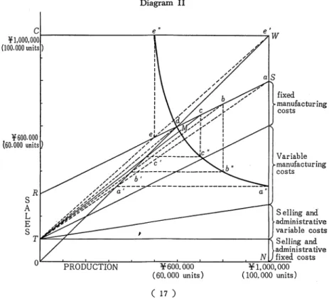
If various production volumes are given in place of y in formula (3') or (R3'), break-even sales point on the various production volumes can be easily
Diagram II
C e'
¥ 1 , 0 0 0 , o o o i - - - . - - - . : . , . w (100.000 units)
¥600.000 (60.000 units
s R
fixed manufacturing costs
Variable manufacturing costs
A L S eI!ing and.
E administrative
S variable costs
T~=-;z:.:..__ _ _ _ _ _ ___:_ _ _ _ _ _ _ _ _ _ _ _ _ -k' Selling and
0 PRODUCTION ¥600.000
( 60. 000 units) ( 17)
administrative N fixed. costs
¥1,000,000 (100. 000 units)
determined, and the break-even sales line in diagram I could be plotted by formula (3') or (R3'). However, if formulas (3') and (R3') are not used, the break-even sales line can be plotted as in the following diagram II. If a line. (for instance, ST line) is drawn from an interesecting point between the total costs RS line and a certain production volume to the point T to be reco- vered at the sales volume 0, break-even sales is a point where the line is interesected by the sales revenue OW line. For example, if the line bT is drawn from an intersecting point b between the total costs RS line and b production volume (80.000 units) to point T, break-even sales volume is the point b' ( 40.000 units) on line bT which intersects the sales revenue OW line.
Then, point b" (production volume=80.000, sales volume=40.000) could be looked for as the vertex of a right-angled triangle (6,b'b"b).
If each y (production volume) is given a certain quantity, each break-even sales volume can be found at eachy (production volume). Subsequently, the break-even sales e"a" line could be plotted in diagram II.
IV BREAK-EVEN ANALYSIS IN STANDARD ABSORTION COSTING Break-even analysis in standard absorption costing, using the condition that under- or over- absorbed fixed overhead costs are assumed to be period cost or period revenue, is discussed in various articles, e.g., Professor A_merman (a paper in 1954), Professor Brummet (a book in 1957), Professor Patrick (a paper in 1958), Professors Henderson and Brock (a paper in 1964), Professors Terrill and Patrick (a book in 1965), etc.1
1. ' © Gilbert Amerman, "Facts About Direct- Costing for Profit Determination,"
Accounting Researchi, Vol. V, No. 2 (April, 1954).
® R. Lee Brummet, Overhead Costing: The Costing of Manufactured Products (Ann Arbor: Bureau of Business Research, School of Business Administration, The
University of Michigan, 1957).
® Albert W. Patrick, "Some Observations on the Break-Even Chart", Acc,unting Review, Vol. XXIX, No. 4 (October, 1958).
© Porter W. Henderson and Horace R. Brock, "Imbalanced Volume Break-even Analysis for Use with the Comprehensive Budget Program," Butlgeting, Vol. XIII,.
No. 2, (November, 1964).
® William A. Terrill and Albert W. Patrick, Cost Accounting for Management (New York: Holt, Rinehart and Winston, Inc., 1965).
® We have some papers on this problem in Japan.
( 18 )
BREAK-EVEN ANALYSIS AND FIXED OVERHEAD COSTING (Suemasa) 204
They approached break-even analysis by using numerical formulas or dia- grams. However, I intend to approach break-even analysis by different formula of the conventional break-even type. My modified formulas of the conventional break-even formula give the same results. The method of using the modified formula makes the most of the fundamental device of the con- centional break-even formula. That is, I intend to utilize special meaning numerator and denominator of the break-even formula. And then, this method can be easily compared with any other break-even analysis in each costing system, i.e., in actual absorption costing, or in standard absorption costing, or in direct costing.
Namely, the period-fixed cost of the numerator and the contribution margin ratio of the denominator in this break-even formula under the standard absorp- tion costing can be compared with that of other break-even formula in other costings. And my method differs from their formula and diagram analysis in some points, and must pay attention to their distinctive features as follows:
1. Their break-even analysis are based on a standard absorption costing that is used as a 100% capacity (or activity) base for their selected capacity (or activity). For example, Professor Brummet,2 and Proefessors Henderson and Brock's3 methods based upon a 100% base for the level of normal capacity, Professors Terrill and Patrick's method is based on a 100% base for annual practical capacity.4 Consequently, their break- even sales line is only one line.
2. Their methods assume a less than 100% capacity base, except in the case of Professors Henderson and Brock, where a certain under-absorbed fixed cost sometimes occurs. Then, the under-absorbed fixed cost is assumed to be period cost. Consequently, none of the methods except for that of Professors Henderson and Brock, show any occurrence of over- absorbed fixed cost, because they don't have any case of more than 100% capacity base. However, in the case of Professors Henderson and Brock, favorable volume variances occur, for there is more than 100%
2. R. Lee Brummet, o;. cit., p. 91.
3. Porter W. Henderson and Horace R. Brock, op. cit., p. 15.
4. William A. Terrill and Albert W. Patrick, op. cit., p. 543.
( 19)
normal capacity base.5 Therefore, I intend to discuss standard absorption costing under each concept of capacity (or activity) and how this costing relates to the break-even sales (or xn). I will co~sider standard absorption costing under various concepts of capacity (or activity) that are assumed to have occurred in my cases. Then, in some cases, over-absorbed fixed overhead cost will be treated in the break-even analysis, and it will be assumed that over-absorbed fixed overhead cost is period revenue like other income. I want to look at the allocation procedure of fixed overhead cost in standard absorption costing.
Standard fixed overhead burden rate in standard absorption costing is determined by th_e following formula:
budgeted fixed overhead costs standard capacity (or activity) level
The budgeted fixed overhead costs in the numerator are assumed in the earlier sections to coincide with the actual fixed. overhead cost or estimated fixed overhead cost. Then, the procedure in determining the standard fixed overhead burden rate is the selection of a certain standard level of capacity (or activity) in the denominator. Generally speaking, there are four levels of capacity (or activity).
( 1 ) Theoretical maximum or full capacity (ideal standard), based on maximum physical plant capacity.
( 2) Practical capacity (attainable standard), based on the practically '. attainable production level.
( 3) Normal or average capacity (average [sales] of several years), based on the ability to sell and produce in several periods (over the long run).
( 4) Budgeted or expected (actual) capacity (expected level of perform- ance), based on the expected sales in the coming period ( over the short run).6
· 5. Porter W. Henderson and Horace R. Brock, op. cit., p. 15.
6. © Morton Backer and Lyle E. Jacobsen; Cost Accounting, A Managerial Approach (New York: McGraw-Hill Book Co., 1964), p. 289.
® R. Lee Brummet, op. cit., pp. 17-18, pp. 62-66.
® Carl L. Moore and Robert K. Jaedicke, Managerial Accounting (Cincinnati:
South-Western Publishing Co., 1963), p. 318.
© Glenn A. Welsch, op. cit., p. 187.
( 20)
BREAK-EVEN ANALYSIS AND FIXED OVERHEAD COSTING (Suemasa) 202
For profit reporting. Theoretical maximum capacity basis may be ruled out as a practical procedure. This basis is used only as a point of.departure in the calculation of other activity (or capacity) level concepts. The other three bases (2), (3), (4) are frequently used for profit determination or profit planning. For example, Professor Haseman stated that the concept of prac- tical capacity or normal capacity is most commonly used with a standard cost system. 7 But there are numerous theories (and opinions) as to what level of capacity ( or activity) should be used.
Professor Neuner stated that "A survey by the N. A. A. indicated that 60 per cent of companies use practical capacity in their budgeting, ... ".8
Professor Bierman stated that "Since practical capacity is so difficult to define, normal activity is frequently used. "9
Professors Backer and Jacobsen stated that "The most commonly used basis for setting factory overhead rate is normal capacity."10
Professors Matz, Curry and Frank stated that "Determination of estimates used in deriving a burden rate depends on whether a long or short range viewpoint is adopted: i.e., whether the activity level used is (a) n9rmal capa- city or .(b) expected actual capacity."11
Professor Welsch stated from a viewpoint of budgeting that "Capacity variance is measured from· expected actual rather than plant capacity, prac- tical capacity or normal capacity."lB
And yet, many writers generally advocate the normal capacity as a basis. •
If it is adopted as the normal capacity basis, Professors Moore and J aedicke indicate that, "Normal capacity is not easy to define."13
7. Wilber C. Haseman, Management Uses of Accounting (Boston: Allyn and Bacon, Inc., 1963), p. 554.
8. John J. W. Neuner, Cost Accounting: Principles and Practice (Howemood, Ill.:
Richard D. Irwin, Inc., 1962), p. 595.
9. Harold Bierman, Topics in Cost Accounting and Decisions (New York: McGraw-Hill Book Co., 1963), p. 11.
10. Morton Backer and Lyle E. Jacobsen, op. cit., p. 290.
11. Adolph Matz, Othel J. Curry and George W. Frank, Cost Accounting: Manage- ment's Operational Tool for Planning, Control, and Analysis (Cincinnati: South-Western Publishing Co., 3d ed. 1962), p. 290.
12. Glenn A. Welsch, op. cit., p. 415.
13. Carl L. Moore and Robert K. Jaedicke op.·cit., p. 318.
(.21)
That is, a concrete quantity in normal capacity basis is quite difficult to define. ~rofessor Welsch stated that "Authorities are not in agreement with respect to preferable rate."14 Thus, there are many cases of selection on the capacity basis. However, the selection depends upon the following elements.
First, selection depends on whether or not management has carefully con- sidered the effect and nature of volume variance (idle capacity variance or excess capacity variance).15 Second, selection depends on whether the mech- anism of profit planning and budgeting in relation to the selection of capacity basis is in line with the mechanism of costing system for control purposes.
Therefore, selection depends primarily upon the preference of the management.
I intend to give many examples of all levels of capacity, but mainly the fore- going four capacities. In this way, I hope to show how large a break-even sales ( or x") is influenced by the fixed overhead costs allocated on the basis of each capacity.
First, I want to assume that idle capacity variance in every case is period cost, and excess capacity variance is period revenue. The example which follows was taken from those giv~ by Professor Gillespie, Professor Brummet, and Professor Neuner, with respect to each capacity basis on the comparative income statements. That is, Professor Gillespie has assumed that practical capacity is 100% base, and that average (normal) capacity is 90% against the practical capacity (100%). While expected capacity is 80% against the practical capacity (100%).1&
Professor Brummet has assumed that practical capacity is 100% base, and that average or expected activity is 75% against the practical capacity (100%). 17 Professor Nuener has described practical. capacity defined in a scope of 75%- 85% on the theoretical capacity. 18 Therefore, I have assumed as follows:
Practical capacity
Normal (average) capacity Expected capacity A 14. Glenn A. Welsch, op. cit., p. 187.
15. Carl L. Moore and Robert K. Jaedicke, op. cit., p. 318.
100%
90%
80%
16. Cecil Gillespie, Standard and Direct Costing (Englewood Cliffs, N. J.: Prentice-
Hall, Inc., 1962), pp. 94-95. .
17. R. Lee Brummet, op. cit., p. 35.
18. John J. W. Neuner; op. cit., pp. 533-534.
( 22)
Comparative Income Statements ( under each capacif:)I or activif:)I level)
The base of capactity or activity Expected Capacity B Expected Capacity A Normal or Average Capacity Practical Capacity (100%) Theoretical Capacity
(!) Volume units 60,000 untis 70,000 units 80,000 units 90,000 units 100,000 units 110,000 units 120,000 units 130,000 units
® Volume percents (base 100,000 units) 60% 70% 80% 90% 100% 110% 120% 130%
Sales (60,000 units) @¥ 10.00 600,000 600,000 600,000 600,000 600,000 600,000 600,000 600,000
Cost of goods sold
Beginning inventory ( 0 units) 0 0 0 0 0 0 0 0
Standard variable production costs (80,000 units) @¥ 3.50 280,000 280,000 280,000 280,000 280,000 280,000 280,000 280,000
Standard fixed production costs ( II II ) 266,264 230, 568 200,000 177,776 160,000 145,448 133,328 123,072
Cost of goods available for sale ( II II ) 546,664 510,568 480,000 457, 776 440,000 425,448 413,338 403,072
Ending inventory (20,000 units) 136,666 127,142 120,000 114,444 110,000 106,362 103,332 100, 768
Cost of goods sold (60,000 units) 409,998 383,426 360,000 343,332 330,000 319,086 309,996 302,304
Gross manufacturing margin 190,002 216,574 240,000 256,668 270,000 286,814 290,004 297,696
Volume variance
Unfavorable balance (debit) 0 0 0 22,224 40,000 54,552 66,672 76,928
Favorable balance (credit) 66,664 30,568 0 0 0 0 0 0
- - - -
Net manufacturing margin 256,666 247,142 240,000 234,444 230,000 226,262 223,332 220,768
Selling and Administrative costs
Variable cost componets (60,000 units) @¥ 1.50 90,000 90,000 90,000 90,000 90,000 90,000 90,000 90,000
Fixed cost components ( " 11 ) (Total ¥100,000) 100,000 190,000 100,000 190,000 100,000 190,000 100,000 190,000 100,000 190,000 100,000 190,000 100,000 190,000 100,000 190,000
Net income 66,000 57,142 50,000 44,444 40,000 36,262 33,332 30,768
Break-even sales point ¥ 200,000 ¥ 324,009 ¥ 400,000 ¥ 440,000 ¥ 466,666 ¥ 485,722 ¥ 500,000 ¥ 511,116
[Footnote]
Standard fixed production costs calculations
Fixed production cost components (total) ¥ 200,000 (a) ¥ 200,000 (a) ¥ 200,000 (a) ¥ 200,000 (a) ¥ 200,000 (a) ¥ 200,000 (a) ¥ 200,000 (a) ¥ 200,000 (a)
The base by volune (standard volune) 60,000 (b) 70,000 (b) 80,000 (b) 90,000 (b) 100,000 (b) 110,000 (b) 120,000 (b) 130,000 (b)
Actual production volume 80,000 (c) 80,000 (c) 80,000 (c) 80,000 (c) 80,000 (c) 80,000 (c) 80,000 (c) 80,000 (c)
Burden rate per unit ¥ 3.3333 (a)+(b) ¥ 2. 8571 (a)+(b) ¥ 2.5000 (a)+ (b) ¥ 2.2222 (a)+ (b) ¥ 2.0000 (a)+(b) ¥ 1. 8181 (a)+(b) ¥ 1. 6666 (a)+ (b) ¥ 1. 5384 (a)+(b) Ending inventory calculation
Stadard variable production. costs (20,000 units) @¥ 3.50 ¥ 70,000 ¥ 70,000 ¥ 70,000 ¥ 70,000 ¥ 70,000 ¥ 70,000 ¥ 70,000 ¥ 70,000
Standard fixed production costs (20,000 units) ¥ 66,666 @¥3. 3333 ¥ 57,142 @¥2. 8571 ¥ 50,000 @¥2. 5000 ¥ 44,444 @¥2. 2222 ¥ 40,000 @ 2.0000 ¥ 36,362 @¥1. 8181 ¥ 33,332 @ 1. 6666 ¥ 30,768 @¥1. 5384