A center manifold reduction of the Kuramoto-Daido model with a

A center manifold reduction of the Kuramoto-Daido model with a

phase-lag

Institute of Mathematics for Industry, Kyushu University / JST PRESTO, Fukuoka, 819-0395, Japan

Hayato CHIBA

Sep 11, 2016; Revised Dec 15, 2016 Abstract

A bifurcation from the incoherent state to the partially synchronized state of the Kuramoto-Daido model with the coupling function f(θ) = sin(θ+α

)+

h sin 2(θ+α

) is investigated based on the generalized spectral theory and the center manifold reduction. The dynamical system of the order parameter on a center manifold is derived under the assumption that there exists a center manifold on the dual space of a certain test function space. It is shown that the incoherent state loses the stability at a critical coupling strength K = K

, and a stable rotating partially synchronized state appears for K > K

. The velocity of the rotating state is different from the average of natural frequencies of oscillators when α

̸ = 0.

1 Introduction

Collective synchronization phenomena are observed in a variety of areas such as chemical reactions, engineering circuits and biological populations [10]. In order to investigate such phenomena, a system of globally coupled phase oscillators called the Kuramoto-Daido model [5]

dθ

dt = ω

+ K N

∑

f(θ

− θ

), i = 1, · · · , N, (1.1) is often used, where θ

= θ

(t) ∈ [0, 2π) is a dependent variable which denotes the phase of an i-th oscillator on a circle, ω

∈ R denotes its natural frequency

1

[email protected]

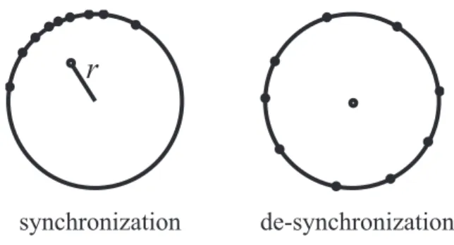
Figure 1: Collective behavior of oscillators.

drawn from some density function g(ω), K > 0 is a coupling strength, and where f (θ) is a 2π-periodic function. The order parameter defined by

r := 1 N

∑

e

, i = √

− 1 (1.2)

is used to measure the amount of coherence in the system; if r is nearly equal to zero, oscillators are uniformly distributed (called the incoherent state), while if r > 0, the synchronization occurs, see Fig. 1. In the last few decades, the existence, stability and bifurcations of the synchronization have been well studied, however, the coupling function f(θ) was still restricted to some specific form.

In this paper, the onset of the synchronization of the continuous limit (thermodynamics limit) for the following model

dθ

dt = ω

+ K N

∑

( sin(θ

− θ

+ α

) + h · sin 2(θ

− θ

+ α

) )

, (1.3) will be considered, where α

, α

are phase lags and h is a parameter which controls the strength of the second harmonic. For the continuous limit of the system given in Sec.2, a bifurcation from the incoherent state (the de- synchronous state) to the partially synchronized state will be investigated based on the generalized spectral theory.

When h = α

= 0, the model is well known as the original Kuramoto model. For a bifurcation of the partially synchronized steady state in this case, it has been proved (the Kuramoto conjecture) that :

Suppose that the density function g(ω) for natural frequencies is an even and unimodal function, and satisfies a certain regularity condition.

(i) (Instability of the incoherent state). When K > K

:= 2/(πg(0)),

then the incoherent state of the continuous limit is unstable.

(ii) (Local stability of the incoherent state). When 0 < K < K

, the incoherent state is locally asymptotically stable with respect to a certain topology.

(iii) (Bifurcation). There exists a positive constant ε

such that if K

− ε

<

K < K

+ ε

and if an initial condition is close to the incoherent state (with respect to a certain topology), the order parameter is locally governed by the dynamical system

dr

dt = const.

(

K − K

+ πg

(0)K

16 r

)

r + O(r

). (1.4) In particular, when K > K

, the order parameter tends to the positive constant expressed as

r =

√ − 16 πK

g

(0)

√ K − K

+ O(K − K

), (1.5)

as t → ∞ .

In Chiba [1, 2], this result is proved based on the generalized spectral theory [3] under the assumption that g(ω) has an analytic continuation near the real axis. In Dietert [6] and Fernandez et al. [7], they proved a similar result with a weaker assumption for g(ω). See these references for the precise assumptions for g(ω) and for the topologies for the stability.

In [1], this result was extended to the case α

= α

= 0 and h < 1 (i.e. the coupling function is f (θ) = sin θ + h sin 2θ). With the aid of the generalized spectral theory, the dynamics of the order parameter on a center manifold was shown to be

dr

dt = const.

(

K − K

− K

Ch 1 − h r

)

r + O(r

),

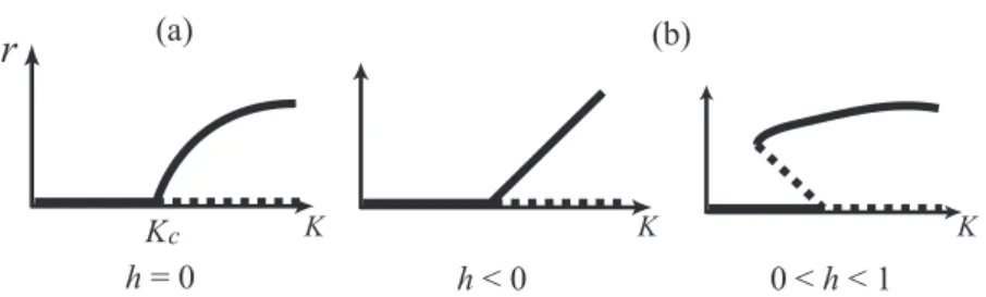
where C is a certain negative constant. As a result, a bifurcation diagram of r is given as Fig.2. When h = 0, the synchronous state bifurcates through the pitchfork bifurcation, though when h ̸ = 0, it is a transcritical bifurcation.

Omel’chenko et al.[9] have investigated a bifurcation diagram for the case h = 0, α

̸ = 0 by the self-consistent approach and numerical simulation.

They found that under the synchronized state, the average velocity of oscil- lators is different from the average of their natural frequencies because of the phase-lag α

.

The purpose in this paper is to derive the dynamics of the order param-

eter for the system (1.3) for a certain parameter region (α

, α

, h). To this

end, we need four assumptions (A1) to (A4) given after Section 3. Here, we

Figure 2: Bifurcation diagrams of the order parameter for (a) f (θ) = sin θ and (b) f(θ) = sin θ + h sin 2θ. The solid lines denote stable solutions, and the dotted lines denote unstable solutions.

give a rough explanation of these assumptions.

(A1) We assume that cos α

> 0 so that the interaction between oscillators through the coupling sin(θ + α

) is an attractive coupling. Further, we as- sume that sin(θ + α

) in the coupling function is stronger than the second harmonic h sin 2(θ +α

) in a certain sense. When α

= 2α

, this is equivalent to h < 1.

(A2) We assume that the density g(ω) of natural frequencies is an analytic function near the real axis. This is the essential assumption to apply the generalized spectral theory.

(A3) We will show that at a bifurcation value K = K

, one of the general- ized eigenvalues λ

of a certain linear operator obtained by the linearization of the system lies on the point iy

on the imaginary axis. We assume that λ

is a simple eigenvalue.

(A4) We assume that as K increases, λ

transversally gets across the imag- inary axis at the point iy

from the left to the right.

See after Section 3 for the precise statements for these assumptions. If g(ω) is an even and unimodal function, (A3) is automatically satisfied, though we do not assume it in this paper. The main results in the present paper are;

Theorem 1.1 (Instability of the incoherent state).

Suppose (A1) and g(ω) is continuous. There exists a number ε > 0 such that when K

< K < K

+ ε, the incoherent state is linearly unstable (the value of K

will be given in Section 3).

Theorem 1.2 (Local stability of the incoherent state).

Suppose (A1) and (A2). When 0 < K < K

, the incoherent state is linearly asymptotically stable in the weak sense (see Section 4 for the weak stability).

For a bifurcation, our result is divided into two cases, h = 0 and h ̸ = 0

because types of bifurcations of them are different. As is shown in Fig.2, it is a pitchfork bifurcation when h = 0, while it is a transcritical bifurcation when h ̸ = 0. In this paper, we formally apply the center manifold reduction without a proof of the existence of a center manifold. In Chiba [2], the existence of a center manifold was shown when h = α

= 0 and g is the Gaussian. To prove the existence of center manifolds for a wide class of evolution equations within the setting of the generalized spectral theory is an important challenging work.

Theorem 1.3 (Bifurcation h = 0).

Suppose (A1) to (A4) hold. There exists a positive constant ε

such that if K

− ε

< K < K

+ ε

and if an initial condition is close to the incoherent state, the order parameter is locally governed by the dynamical system

dr

dt = Re(p

)r (

K − K

+ Re(p

) Re(p

) r

)

+ O(r

), (1.6) where p

and p

are certain complex constants given in Section 6. The equation has the fixed point

r

=

√

− Re(p

) Re(p

) · √

K − K

+ O(K − K

). (1.7) The assumption (A4) implies Re(p

) > 0. Thus, if Re(p

) < 0, the bifurcation is supercritical; the fixed point exists for K > K

and is stable. If Re(p

) >

0, the bifurcation is subcritical; the fixed point exists for K < K

and is unstable.

Theorem 1.4 (Bifurcation h ̸ = 0).

Suppose (A1) to (A4) hold. There exists a positive constant ε

such that if K

− ε

< K < K

+ ε

and if an initial condition is close to the incoherent state, the order parameter is locally governed by the dynamical system

dr

dt = Re(p

)r (

K − K

+ Re(p

) Re(p

) r

)

+ O(r

), (1.8) where p

and p

are certain complex constants given in Section 6. The equation has the fixed point

r

= − Re(p

)

Re(p

) · (K − K

) + O((K − K

)

). (1.9) The assumption (A4) implies Re(p

) > 0. Thus, if Re(p

) < 0, the bifurcation is supercritical; the fixed point exists for K > K

and is stable. If Re(p

) >

0, the bifurcation is subcritical; the fixed point exists for K < K

and is

unstable.

Theorem 1.5 (The average velocity).

The complex order parameter (see Eq.(2.1) and (2.2)) under the partially locked state shown in Theorems 1.3 and 1.4 is given by

η

(t) = r

e

· e

(1 + O(r

)),

where r

is a number given in Theorems 1.3 and 1.4, respectively, for h = 0 and h ̸ = 0. Hence, the average velocity of locked oscillators is approximately given by y

(see (A3) and (A4) for the definition of y

). When g(ω) is an even and unimodal function and if α

is small, y

is given by

y

= − g(0)

H[g]

(0) α

+ O(α

), (1.10) where H[g] is a Hilbert transform of g, see Lemma 3.1 and Example 3.6.

When α

= α

= 0, Theorems 1.3 and 1.4 recover the results of [1, 2], and when h = 0, Theorem 1.3 coincides with the result in [9].

2 The continuous model

For the finite dimensional Kuramoto-Daido model (1.1), the k-th order pa- rameter is defined by

ˆ

η

(t) := 1 N

∑

e

. (2.1)

By using it, Eq.(1.1) is rewritten as dθ

dt = ω

+ K

∑

f

η ˆ

(t)e

, f (θ) :=

∑

f

e

. This implies that the flow of θ

is generated by the vector field

ˆ

v = ω

+ K

∑

f

η ˆ

(t)e

.

Thus, the continuous model of Eq.(1.1) is the equation of continuity of the

form 

 

 

 



 

 

 



∂ρ

∂t + ∂

∂θ (ρv) = 0, ρ = ρ(t, θ, ω), v := ω + K

∑

f

η

(t)e

, η

(t) :=

∫

R

∫

0

e

ρ(t, θ, ω)g(ω)dθdω.

(2.2)

Here, g(ω) is a given probability density function for natural frequencies, and the unknown function ρ = ρ(t, θ, ω) is a probability measure on [0, 2π) parameterized by t, ω ∈ R . It is known that a solution of Eq.(1.1) converges to that of Eq.(2.2) as N → ∞ in some probabilistic sense [4]. Our goal is to investigate the dynamics of η

(t), which is a continuous version of Kuramoto’s order parameter (1.2). Roughly speaking, ρ(t, θ, ω) denotes a probability that an oscillator having a natural frequency ω is placed at a position θ. The trivial solution ρ = 1/(2π) of the system is a uniform distribution on the circle, which is called the incoherent state (de-synchronous state). In this case, η

= 0 for all l = ± 1, ± 2, · · · . We will show that a nontrivial stable solution such that | η

| > 0 bifurcates from the incoherent state.

Setting the Fourier coefficients Z

(t, ω) :=

∫

0

e

ρ(t, θ, ω)dθ yields the system of evolution equations of Z

as

dZ

dt = ijωZ

+ ijKf

η

+ ijK ∑

l̸=j

f

η

Z

. (2.3) Indeed, we have

dZ

dt = −

∫

0

e

∂

∂θ (ρv)dθ

= ij

∫

e

ρ(ω + K

∑

f

η

e

)dθ

= ijωZ

+ ijK

∑

f

η

Z

.

Since Z

≡ 1 because of the normalization ∫

0

ρ(t, θ, ω)dθ = 1, we obtain Eq.(2.3). The trivial solution Z

≡ 0 (j = ± 1, ± 2, · · · ) corresponds to the in- coherent state. In what follows, we consider only the equations for Z

, Z

, · · · because Z

is the complex conjugate of Z

.

3 The transition point formula and linear in- stability

To investigate the stability of the incoherent state, we consider the linearized

system. Let L

( R , g(ω)dω) be the weighted Lebesgue space with the inner

product

(ϕ, ψ) =

∫

R

ϕ(ω)ψ (ω)g(ω)dω.

Put P

(ω) ≡ 1 ∈ L

( R , g(ω)dω). We define the one-dimensional integral operator P on L

( R , g(ω)dω) to be

( P ϕ)(ω) =

∫

R

ϕ(ω)g(ω)dω = (ϕ, P

) · P

(ω). (3.1) Then, the order parameters are written by

η

(t) =

∫

R

Z

(t, ω)g(ω)dω = P Z

. (3.2) Note that the term η

Z

= ( P Z

)Z

in Eq.(2.3) is a nonlinear term of Z

, Z

, · · · when j ̸ = l. Hence, the linearized system of Eq.(2.3) around the incoherent state is given by

dZ

dt = T

Z

:= (ijω + ijKf

P )Z

, j = 1, 2, · · · (3.3) Let us consider the spectra of linear operators T

. The multiplication operator ϕ(ω) 7→ ωϕ(ω) on L

( R , g(ω)dω) is self-adjoint. The spectrum of it consists only of the continuous spectrum given by σ

(ω) = supp(g) (the support of g). Therefore, the spectrum of the multiplication by ijω lies on the imaginary axis; σ

(ijω) = ij · supp(g) (later we will suppose that g is analytic, so that σ

(ijω) is the whole imaginary axis). Since P is compact, it follows from the perturbation theory of linear operators [8] that the continuous spectrum of T

is given by σ

(T

) = ij · supp(g), and the residual spectrum of T

is empty.

When f

̸ = 0, eigenvalues λ of T

are given as roots of the equation

∫

R

1

λ − ijω g(ω)dω = 1 ijKf

, λ / ∈ σ

(T

). (3.4) Indeed, the equation (λ − T

)v = 0 provides

v = ijKf

(v, P

)(λ − ijω)

P

.

Taking the inner product with P

, we obtain Eq.(3.4). If λ is an eigenvalue of T

, the above equality shows that

v

(ω) = 1

λ − ijω (3.5)

is the associated eigenfunction. This is not in L

( R , g(ω)dω) when λ is a purely imaginary number. Thus, there are no eigenvalues on the imaginary axis. Putting λ = x + iy in Eq.(3.4) provides

 

 

 



∫

R

x

x

+ (y − jω)

g(ω)dω = − Im(f

) jK | f

|

,

∫

R

y − jω

x

+ (y − jω)

g(ω)dω = Re(f

) jK | f

|

,

which determines eigenvalues of T

. In what follows, we restrict our problem to the model (1.3), for which the coupling function is given by f(θ) = sin(θ + α

) + h sin 2(θ + α

). In this case, we have

f

= 1

2 (sin α

− i cos α

), f

= h

2 (sin 2α

− i cos 2α

), (3.6) and f

= 0 for j ̸ = 1, 2. The spectrum of the operator T

for j ̸ = 1, 2 consists of the continuous spectrum on the imaginary axis. The eigenvalues of T

and T

are determined by the equations

 

 

 



∫

R

x

x

+ (y − ω)

g(ω)dω = 2

K cos α

,

∫

R

y − ω

x

+ (y − ω)

g(ω)dω = 2

K sin α

,

(3.7)

and 

 



 



∫

R

x

x

+ (y − 2ω)

g(ω)dω = h

K cos 2α

,

∫

R

y − 2ω

x

+ (y − 2ω)

g(ω)dω = h

K sin 2α

,

(3.8) respectively.

Let us study the properties of Eq.(3.4) for j = 1 or equivalently Eq.(3.7).

Define a function D(λ) to be D(λ) =

∫

R

1

λ − iω g(ω)dω. (3.9)

The next lemma follows from well known properties of the Poisson integral and the Hilbert transform. See [11] for the proof.

Lemma 3.1. Suppose g(ω) is smooth at ω = y. Then, the equality

λ→

lim

D

(λ) = ( − 1)

n! · lim

λ→+0+iy

∫

R

1

(λ − iω)

g(ω)dω

= 1

i

· lim

λ→+0+iy

∫

R

1

λ − iω g

(ω)dω

= 1

i

( πg

(y) − iπH[g

](y) )

holds for n = 0, 1, 2, · · · , where λ → +0 + iy implies the limit to the point iy ∈ i R from the right half plane and H[g] denotes the Hilbert transform defined by

H[g](y) = − 1 π p.v.

∫

R

1

ω g(ω + y)dω

= − 1 π lim

ε→+0

∫

ε

1

ω (g(y + ω) − g(y − ω)) dω.

Lemma 3.2. Suppose K > 0 and cos α

> 0. Then, (i) If an eigenvalue λ of T

exists, it satisfies Re(λ) > 0.

(ii) If K > 0 is sufficiently large, there exists at least one eigenvalue λ near infinity on the right half plane.

(iii) If K > 0 is sufficiently small, there are no eigenvalues of T

.

Proof. Part (i) is obvious from the first equation of (3.7). For (ii), Eq.(3.4) gives 1/λ + O(1/λ

) = 1/iKf

when | λ | is large. Rouch´ e’s theorem proves that Eq.(3.4) has a root λ ∼ iKf

if K > 0 is sufficiently large. To prove (iii), we can show that the left hand side of the first equation of Eq.(3.7) is bounded for any x, y ∈ R , while the right hand side is not as K → +0. See [2] for the detail. □

Eq.(3.7) combined with Lemma 3.1 yields

 

 

 



x

lim

∫

R

x

x

+ (y − ω)

g(ω)dω = 2

K cos α

= πg(y),

x

lim

∫

R

y − ω

x

+ (y − ω)

g(ω)dω = 2

K sin α

= πH[g](y).

Thus, we obtain tan α

· g(y) = H[g](y). Let y

, y

, · · · be roots of this equation, and put K

= 2 cos α

/(πg(y

)). The pair (y

, K

) describes that some eigenvalue λ = λ

(K) of T

on the right half plane converges to the point iy

on the imaginary axis as K → K

+ 0. Since Re(λ) > 0, the eigenvalue λ

(K) is absorbed into the continuous spectrum on the imaginary axis and disappears at K = K

. Suppose that y

satisfies sup

{ g(y

) } = g(y

) and put

K

= inf

j

{ K

} = 2 cos α

πg(y

) . (3.10)

In this section, we need not assume that y

satisfying sup

{ g(y

) } = g(y

) is unique, although we will assume it in Sec.6. We have proved that

Proposition 3.3. Suppose g(ω) is continuous and cos α

> 0. Then,

(i) The continuous spectrum of T

is given by σ

(T

) = i · supp(g) ⊂ i R .

(ii) Eigenvalues of T

are given by roots of Eq.(3.4) for j = 1. If it exists,

Re(λ) > 0.

(iii) Any eigenvalue converges to some point iy

on the imaginary axis as K → K

+ 0 > 0 and disappears at K = K

.

(iv) When 0 < K < K

, T

has no eigenvalues on the right half plane.

In what follows, λ

(K) denotes the eigenvalue of T

satisfying λ

→ +0 + iy

as K → K

+ 0. The following formulae will be used later.

Lemma 3.4. The equalities

D(iy

) := lim

λ→+0+iyc

D(λ) = 1 iK

f

, dλ

dK

K=Kc

= − 1

iK

f

D

(iy

) hold.

Proof. The first one follows from Eq.(3.4) and the definition of (y

, K

). The derivative of Eq.(3.4) as a function of λ gives

D

(λ) = − 1 iK(λ)

f

dK dλ . This proves the second one. □

The eigenvalues of T

are calculated in a similar manner. The limit x → +0 for Eq.(3.8) provides

 

 

 



x

lim

∫

R

x

x

+ (y − 2ω)

g(ω)dω = h

K cos 2α

= 1

2 πg(y/2),

x

lim

∫

R

y − 2ω

x

+ (y − 2ω)

g(ω)dω = h

K sin 2α

= 1

2 πH [g](y/2).

Let y

, y

, · · · be roots of the equation tan 2α

· g(y/2) = H[g](y/2). Define K

= 2h cos 2α

/(πg(y

/2)) and K

= inf

{ K

} . Then, T

satisfies a similar statement to Proposition 3.3.

In what follows, we assume the following;

(A1) cos α

> 0 and K

< K

.

The assumption cos α

> 0 shows that eigenvalues of T

lie on the right

half plane (Lemma 3.2). The assumption K

< K

implies that the eigen-

value λ

of T

still exists on the right half plane after all eigenvalues of T

disappear as K decreases. In other words, as K increases from zero, the

eigenvalue λ

of T

first emerges from the imaginary axis before some eigen- value of T

emerges. When α

= 2α

, K

< K

is equivalent to the condition h < 1 (i.e. the first harmonic sin θ dominates the second harmonic h sin 2θ for the attractive coupling between oscillators).

Theorem 3.5 (Instability of the incoherent state).

Suppose (A1) and g (ω) is continuous. If 0 < K < K

, the spectra of opera- tors T

, T

, · · · consist only of the continuous spectra on the imaginary axis.

There exists a small number ε > 0 such that when K

< K < K

+ ε, the eigenvalue λ

of T

lies on the right half plane. Therefore, the incoherent state is linearly unstable.

This suggests that a first bifurcation occurs at K = K

and the eigenvalue λ

of T

plays an important role to the bifurcation.

Example 3.6. In this example, suppose that g is an even function. Then, the Hilbert transform H[g] is odd. In particular H[g](0) = 0.

(i) Suppose that α

̸ = nπ. Then, y = 0 does not satisfy the equation tan α

· g(y) = H[g](y) unless g(0) = 0. If y

̸ = 0 satisfies this equation,

− y

does not unless g(y

) = 0. Hence, a Hopf bifurcation does not occur at K = K

. We will consider this situation in this paper.

(ii) Suppose that α

= 0. Then, y = 0 is a root of the equation tan α

· g(y) = H[g](y). If y

̸ = 0 is a root, so is − y

. If further suppose that g(ω) is a unimodal function (g(0) > g(y

)), y

= 0 and the eigenvalue λ

emerges at the origin at K = K

. As a result, a pitchfork (h = 0) or a transcritical (h < 1) bifurcation occurs at K = K

, see Fig.2. If g(ω) is bimodal, g(0) < g(y

) = g( − y

) in general. As a result, a pair of eigenvalues emerges from the imaginary axis at K = K

and a Hopf bifurcation seems to occur. In this paper, we are interested in the effect of phase-lag α

̸ = 0, and thus a Hopf bifurcation is not considered.

When g(ω) is even and unimodal, the implicit function theorem shows that y

is given by

y

= − g(0)

H[g]

(0) α

+ O(α

) (3.11) as α

→ 0.

4 Linear stability

When 0 < K < K

, there are no spectra of operators T

, T

, · · · on the

right half plane, while the continuous spectra of them lie on the imaginary

axis. Hence, one may expect that the incoherent state is neutrally stable.

Nevertheless, we will show that the incoherent state is asymptotically stable in a certain weak sense. The key idea is as follows.

For j ≥ 3, T

= ijω is the multiplication operator. Thus, the semigroup is easily obtained as e

= e

. For any ϕ ∈ L

( R , g(ω)dω), e

ϕ is actually neutrally stable with respect to the L

( R , g(ω)dω)-topology; || e

ϕ || = || ϕ || . Let us consider the inner product with another function ψ

(e

ϕ, ψ) =

∫

R

e

ϕ(ω)ψ(ω)g(ω)dω.

It is known as the Riemann-Lebesgue lemma that if the function ϕ(ω)ψ(ω)g(ω) has some regularity, this quantity tends to zero as t → ∞ . In particular if ϕ(ω)ψ(ω)g(ω) is an analytic function, (e

ϕ, ψ) decays to zero exponentially.

Thus, e

ϕ decays to zero in some weak sense.

To be precise, we need the following assumption. Let δ be a positive number and define the stripe region on C

S(δ) := { z ∈ C | 0 ≤ Im(z) ≤ δ } . We assume that

(A2) The density function g (ω) has an analytic continuation to the region S(δ). On S(δ), there exists a constant C > 0 such that the estimate

| g(z) | ≤ C

1 + | z |

, z ∈ S(δ) (4.1) holds.

Let H

be the Hardy space: the set of bounded holomorphic functions on the real axis and the upper half plane. It is a subspace of L

( R , g(ω)dω).

For ψ ∈ H

, set ψ

(z) := ψ(z).

A function f

∈ L

( R , g(ω)dω) parameterized by t is said to be convergent to zero in the weak sense if the inner product (f

, ψ

) decays to zero as t → ∞ for any ψ ∈ H

. Note that P

∈ H

and the order parameter is written as η

(t) = (Z

, P

) = (Z

, P

). This means that it is sufficient to consider the stability in the weak sense for the stability of the order parameter.

For j ≥ 3, we have

(e

ϕ, ψ

) =

∫

R

e

ϕ(ω)ψ(ω)g(ω)dω.

(the conjugate ψ

is introduced to avoid the complex conjugate in the right

hand side). Now a standard technique of function theory shows (e

ϕ, ψ

) =

∫

e

ϕ(ω)ψ(ω)g(ω)dω

= e

∫

R

e

ϕ(ω + iδ)ψ(ω + iδ)g(ω + iδ)dω.

Hence, there is a constant D such that | (e

ϕ, ψ

) | < De

for t > 0 if ϕ, ψ ∈ H

and if g satisfies (A2). Therefore, the trivial solution of the linearized system (3.3) for j ≥ 3 is asymptotically stable in the weak sense.

To prove a similar fact for j = 1, 2, we need the following fundamental lemma.

Lemma 4.1[2, 3]. Let f(z) be a holomorphic function on the region S(δ).

Define a function A[f ](λ) of λ to be A[f](λ) =

∫

R

1

λ − iω f (ω)dω

for Re(λ) > 0. It has an analytic continuation ˆ A[f](λ) from the right half plane to the region − δ ≤ Re(λ) ≤ 0 given by

A[f ˆ ](λ) =

 

 

 



A[f ](λ) Re(λ) > 0 lim

Re(λ)→+0

A[f](λ) Re(λ) = 0

A[f ](λ) + 2πf ( − iλ) − δ ≤ Re(λ) < 0.

(4.2)

Proof. It is verified by using the formulae on the Poisson integral

λ→

lim

A[f ](λ) = πf (y) − iπH [f ](y),

λ→−

lim

A[f ](λ) = − πf (y) − iπH[f ](y),

see Lemma 3.1. This shows that the first line and the third line of Eq.(4.2) coincide with one another on the imaginary axis, and it is continuous on the imaginary axis. Thus, the right hand side of (4.2) is holomorphic. □

It is known that the semigroup e

of an operator T is expressed by the Laplace inversion formula

e

= lim

y→∞

1 2πi

∫

x−iy

e

(λ − T )

dλ, (4.3)

for t > 0 if T is a generator of a C

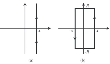
-semigroup [12]. Here, x > 0 is chosen so

that the integral path is to the right of the spectrum of T (see Fig.3(a)). The

next purpose is to calculate the resolvent of our operator T

= iω + iKf

P . Lemma 4.2. The resolvent of T

is given by

(λ − T

)

ϕ = (λ − iω)

ϕ + iKf

1 − iKf

D(λ) ((λ − iω)

ϕ, P

) 1

λ − iω . (4.4) Let λ

be a simple eigenvalue of T

. The projection Π

to the eigenspace of λ

is given by

Π

ϕ = − 1

D

(λ

) ((λ

− iω)

ϕ, P

) 1

λ

− iω . (4.5)

Proof. Put R = (λ − T

)

. We have

(λ − T

)Rϕ = (λ − iω − iKf

P )Rϕ = ϕ.

This provides

Rϕ = (λ − iω)

ϕ + iKf

(Rϕ, P

)(λ − iω)

P

. (4.6) The inner product with P

yields

(Rϕ, P

) = ((λ − iω)

ϕ, P

) + iKf

(Rϕ, P

)((λ − iω)

P

, P

) (Rϕ, P

) = 1

1 − iKf

D(λ) ((λ − iω)

ϕ, P

).

Substituting this into Eq.(4.6) gives Rϕ.

Next, we calculate Π

ϕ. Let γ be a small simple closed curve enclosing λ

. By the assumption, λ

is a pole of (1 − iKf

D(λ))

of the first order, and (λ − iω)

is regular inside γ (recall that an eigenvalue is a root of 1 − iKf

D(λ) = 0). Hence, the Riezs projection is calculated as

Π

ϕ = 1 2πi

∫

γ

(λ − T

)

ϕdλ

= 1

2πi · iKf

· ((λ

− iω)

ϕ, P

) 1 λ

− iω

∫

γ

dλ

1 − iKf

D(λ) . The residue theorem gives

∫

γ

dλ

1 − iKf

D(λ) = 2πi 1

− iKf

D

(λ

) .

This completes a proof of the lemma. □

Lemma 4.2 provides ((λ − T

)

ϕ, ψ

)

= ((λ − iω)

ϕ, ψ

) + iKf

1 − iKf

D(λ) ((λ − iω)

ϕ, P

) · ((λ − iω)

ψ, P (4.7)

), which is meromorphic in λ on the right half plane. Suppose ϕ, ψ ∈ H

. Due to the fundamental lemma 4.1, ((λ − T

)

ϕ, ψ

) has an analytic continuation, possibly with new singularities, to the region − δ ≤ Re(λ) ≤ 0 (Lemma 4.1 is applied to the factors D(λ), ((λ − iω)

ϕ, ψ

), ((λ − iω)

ϕ, P

) and ((λ − iω)

ψ, P

)). A singularity on the left half plane is a root of the equation

1 − iKf

(D(λ) + 2πg( − iλ)) = 0. (4.8) Such a singularity of the analytic continuation of the resolvent on the left half plane is called the generalized eigenvalue (see Sec.5 for the detail).

Now we can estimate the behavior of the semigroup by using the analytic continuation. We have

(e

ϕ, ψ

) = lim

y→∞

1 2πi

∫

x−iy

e

((λ − T

)

ϕ, ψ

)dλ,

where the integral path is given as in Fig.3 (a). When ϕ, ψ ∈ H

, the integrand ((λ − T

)

ϕ, ψ

) has an analytic continuation to the region − δ ≤ Re(λ) ≤ 0 which is denoted by R (λ).

Lemma 4.3. Fix K such that 0 < K < K

. Take positive numbers ε, R and consider the rectangle shaped closed path C represented in Fig.3 (b). If ε > 0 is sufficiently small, the analytic continuation of ((λ − T

)

ϕ, ψ

) is holomorphic inside C for any R > 0.

If this lemma is true, we have 0 =

∫

e

((λ − T

)

ϕ, ψ

)dλ +

∫

−ε+iR

e

R (λ)dλ +

∫

x+iR

e

((λ − T

)

ϕ, ψ

)dλ +

∫

iR

e

R (λ)dλ +

∫

−iR

e

((λ − T

)

ϕ, ψ

)dλ +

∫

−ε−iR

e

R (λ)dλ.

Due to the assumption (A2), we can verify that four integrals in the second and third lines above become zero as R → ∞ (see Appendix for the proof).

Thus, we obtain

(e

ϕ, ψ

) = lim

R→∞

1 2πi

∫

−ε−iR

e

R (λ)dλ.

Figure 3: Deformation of the integral path for the Laplace inversion formula.

This proves | (e

ϕ, ψ

) | ∼ O(e

) as t → ∞ . We can show the same result for the operator T

.

Theorem 4.4 (Local stability of the incoherent state).

Suppose (A1) and (A2). When 0 < K < K

, (e

ϕ, ψ

) decays to zero exponentially as t → ∞ for any j = 1, 2, · · · and any ϕ, ψ ∈ H

. Thus, the incoherent state is linearly asymptotically stable in the weak sense.

Proof of Lemma 4.3. When 0 < K < K

, T

has no eigenvalues on the right half plane and the imaginary axis, so that ((λ − T

)

ϕ, ψ

) is holomorphic on the right half plane and the imaginary axis. A singularity on the left half plane is a root of Eq.(4.8). Since D(λ) and g( − iλ) are holomorphic, the set of singularities has no accumulation points. Hence, for each R > 0, there are no singularities inside the path C if ε = ε(R) is sufficiently small. Finally, Eq.(4.8) is estimated as 1 = O(1/λ) as | λ | → ∞ in the region − δ ≤ Re(λ) ≤ 0. This means that there exists R

> 0 such that if | λ | > R

, there are no singularities in the region − δ ≤ Re(λ) ≤ 0.

Then, the lemma holds with ε = ε(R

). □

5 The generalized spectral theory

For the study of a bifurcation, we need generalized spectral theory developed

in [3] and applied to the Kuramoto model in [2] because the operator T

has

the continuous spectrum on the imaginary axis (thus, the standard center

manifold reduction is not applicable). In this section, a simple review of the

generalized spectral theory is given. All proofs are included in [2, 3]. We

have already encountered a part of the theory; the analytic continuation of the resolvent and its singularity called the generalized eigenvalue. Here, we will reformulate these concept in more functional-analytic manner.

Let H

be the Hardy space on the upper half plane with the norm

|| ϕ ||

= sup

Im(z)>0

| ϕ(z) | . (5.1)

With this norm, H

is a Banach space. Let H

be the dual space of H

; the set of continuous anti-linear functionals on H

. For µ ∈ H

and ϕ ∈ H

, µ(ϕ) is denoted by ⟨ µ | ϕ ⟩ . For any a, b ∈ C , ϕ, ψ ∈ H

and µ, ξ ∈ H

, the equalities

⟨ µ | aϕ + bψ ⟩ = a ⟨ µ | ϕ ⟩ + b ⟨ µ | ψ ⟩ ,

⟨ aµ + bξ | ϕ ⟩ = a ⟨ µ | ϕ ⟩ + b ⟨ ξ | ϕ ⟩ ,

hold. An element of H

is called a generalized function. The space H

is a dense subspace of L

= L

( R , g(ω)dω) and the embedding H

, → L

is continuous. Then, we can show that the dual (L

)

of L

is dense in H

and it is continuously embedded in H

. Since L

is a Hilbert space satisfying (L

)

≃ L

, we have three topological vector spaces called a Gelfand triplet

H

⊂ L

( R , g(ω)dω) ⊂ H

.

If an element ϕ ∈ H

is included in L

( R , g(ω)dω), then ⟨ ϕ | ψ ⟩ is given by

⟨ ϕ | ψ ⟩ := (ϕ, ψ

) =

∫

R

ϕ(ω)ψ(ω)g(ω)dω.

Our operator T

and the above triplet satisfy all assumptions given in [3]

to develop a generalized spectral theory. Now we give a brief review of the theory. In what follows, we assume (A2).

The multiplication operator ϕ 7→ iωϕ has the continuous spectrum on the imaginary axis; its resolvent is given by (λ − iω)

, and it is not included in L

( R , g(ω)dω) when λ is a purely imaginary number. Nevertheless, we show that the resolvent has an analytic continuation from the right half plane to the left half plane in the generalized sense. We define an operator A(λ) : H

→ H

, parameterized by λ ∈ C , to be

⟨ A(λ)ϕ | ψ ⟩ =

 

 

 



 

 

 

((λ − iω)

ϕ, ψ

), Re(λ) > 0, lim

Re(λ)→+0

((λ − iω)

ϕ, ψ

) Re(λ) = 0, ((λ − iω)

ϕ, ψ

)

+2πϕ( − iλ)ψ( − iλ)g( − iλ) − δ ≤ Re(λ) < 0,

for ϕ, ψ ∈ H

. Due to Lemma 4.1, ⟨ A(λ)ϕ | ψ ⟩ is holomorphic. That is, A(λ)ϕ is a H

-valued holomorphic function in λ. In particular, A(λ) coincides with (λ − iω)

when Re(λ) > 0. Since the continuous spectrum of the multiplication operator by iω is the whole imaginary axis, (λ − iω)

does not have an analytic continuation from the right half plane to the left half plane as an operator on L

( R , g(ω)dω), however, it has a continuation A(λ) if it is regarded as an operator from H

to H

. A(λ) is called the generalized resolvent of the multiplication operator by iω.

The next purpose is to define an analytic continuation of the resolvent of T

in the generalized sense. Note that (λ − T

)

is rearranged as

(λ − iω − iKf

P )

= (λ − iω)

◦ (id − iKf

P (λ − iω)

)

.

Since the analytic continuation of (λ − iω)

in the generalized sense is A(λ), we define the generalized resolvent R (λ) : H

→ H

of T

by

R (λ) := A(λ) ◦ (

id − iKf

P

A(λ) )

,

where P

: H

→ H

is the dual operator of P . For each ϕ ∈ H

, R (λ)ϕ is a H

-valued meromorphic function. It is easy to verify that when Re(λ) > 0, it is reduced to the usual resolvent (λ − T

)

. Thus, R (λ) gives a meromorphic continuation of (λ − T

)

from the right half plane to the left half plane as a H

-valued operator. Again, note that T

has the continuous spectrum on the imaginary axis, so that it has no continuation as an operator on L

( R , g(ω)dω).

A generalized eigenvalue is defined as a singularity of R (λ), namely a singularity of (id − iKf

P

A(λ))

.

Definition 5.1. If the equation

(id − iKf

P

A(λ))µ = 0, − δ ≤ Re(λ) (5.2) has a nonzero solution µ in H

for some λ ∈ C , λ is called a generalized eigenvalue and µ is called a generalized eigenfunction.

It is easy to verify that this equation is equivalent to 1

iKf

=

 



 

D(λ) Re(λ) > 0,

lim

Re(λ)→+0

D(λ) Re(λ) = 0, D(λ) + 2πg( − iλ) − δ ≤ Re(λ) < 0.

(5.3)

When Re(λ) > 0, this is reduced to Eq.(3.4) with j = 1. In this case, µ

is included in L

( R , g(ω)dω) and a generalized eigenvalue on the right half

plane is an eigenvalue in the usual sense. When Re(λ) ≤ 0, this equation

is equivalent to Eq.(4.8). The associated generalized eigenfunction is not included in L

( R , g(ω)dω) but an element of the dual space H

. Although a generalized eigenvalue is not a true eigenvalue of T

, it is an eigenvalue of the dual operator:

Theorem 5.2 [2, 3]. Let λ and µ be a generalized eigenvalue and the associated generalized eigenfunction. The equality T

µ = λµ holds.

Let λ

be a generalized eigenvalue of T

and γ

a small simple closed curve enclosing λ

. The generalized Riesz projection Π

: H

→ H

is defined by

Π

= 1 2πi

∫

γ0

R (λ)dλ.

As in the usual spectral theory, the image of it gives the generalized eigenspace associated with λ

, and it satisfies Π

T

= T

Π

[3].

Let λ = λ

(K ) be an eigenvalue of T

defined in Sec.3. Recall that when K

< K , λ

exists on the right half plane. As K decreases, λ

goes to the left side, and at K = K

, λ

is absorbed into the continuous spectrum on the imaginary axis and disappears. However, we can show that even for 0 < K < K

, λ

remains to exist as a root of Eq.(5.3) because the right hand side of Eq.(5.3) is holomorphic. This means that although λ

disappears from the original complex plane at K = K

, it still exists for 0 < K < K

as a generalized eigenvalue on the Riemann surface of the generalized resolvent R (λ). In the generalized spectral theory, the resolvent (λ − T

)

is regarded as an operator from H

to H

, not on L

( R , g(ω)dω). Then, it has an analytic continuation from the right half plane to the left half plane as H

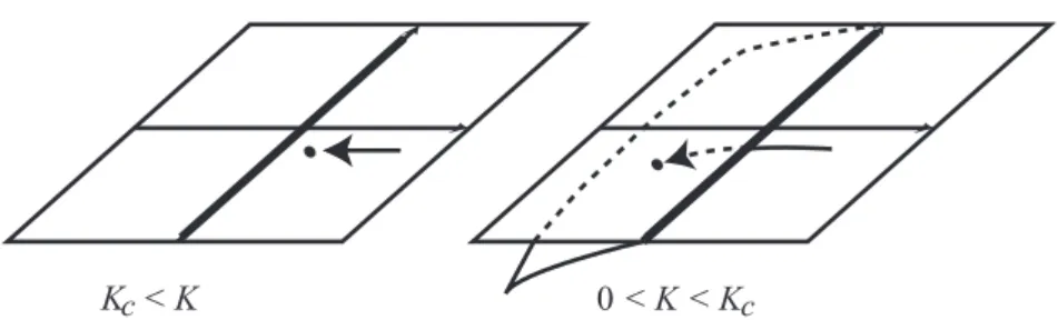
- valued operator. The continuous spectrum on the imaginary axis becomes a branch cut of the Riemann surface of the resolvent. On the Riemann surface, the left half plane is two-sheeted (see Fig.4). We call a singularity of the generalized resolvent on the second Riemann sheet the generalized eigenvalue.

On the dual space H

, the weak dual topology (weak star topology) is equipped; a sequence { µ

} ⊂ H

is said to be convergent to µ ∈ H

if ⟨ µ

| ψ ⟩ ∈ C is convergent to ⟨ µ | ψ ⟩ for each ψ ∈ H

. Recall that an eigenfunction of a usual eigenvalue λ of T

is given by v

(ω) = (λ − iω)

(Eq.(3.5)). A generalized eigenfunction µ

of a generalized eigenvalue iy on the imaginary axis is given by

µ

= lim

λ→+0+iy

1 λ − iω ,

where the limit is considered with respect to the weak dual topology (compare