Generalized State-Dependent Scaling for Local Optimality, Global Inverse Optimality,

(1)

ISSN 1344-8803, CSSE-7 January 31, 2000

Generalized State-Dependent Scaling for Local Optimality, Global Inverse Optimality,

and Global Robust Stability

¹²

Hiroshi Ito y3

y

Department of Control Engineering and Science, Kyushu Institute of Technology 680-4 Kawazu, Iizuka, Fukuoka 820-8502, Japan

Phone: (+81)948-29-7717, Fax: (+81)948-29-7709 E-mail: [email protected]

Abstract: This paper provides a solution to an inverse optimal robust control problem for uncertain nonlinear systems. A new version of robust backstepping is proposed in which inverse optimality is achieved through the selection of generalized state-dependent scaling factors. Like other robust backstepping methods, this design is always successful for uncertain nonlinear systems in strict-feedback form. The class of cost functionals allowed in the inverse optimal design is such that the uncertainty structure and desired level of global robustness can be prescribed a priori. Furthermore, the inverse optimal control law can always be designed such that its linearization is identical to a linear optimal control law for the linearized system with respect to a prescribed quadratic cost functional.

Key Words: Inverse optimal control, Robust backstepping, Global robust stability, State- dependent scaling, Robust control Lyapunov function

1

Technical Report in Computer Science and Systems Engineering, Log Number CSSE-7, ISSN 1344-8803. c

2000 Kyushu Institute of Technology

2

The rst version of the paper was completed by November 1, 1998 during a six months visit to Dept. of Electrical and Computer Engineering, Northwestern University, 2145 Sheridan Road, Evanston, IL 60208-3118, USA. This version was completed on March 4, 1999.

3

Author for correspondence

(2)

1 Introduction

Backstepping methods for the design of robustly stabilizing controllers for uncertain nonlinear systems have been evolving over the past several years. Early results in [1, 2, 3] extended the break- through [4] in nonlinear adaptive control to a class of strict-feedback systems with nonlinear time- varying uncertainties[5]. More recently, these designs have been rened in the context of an inverse optimal robust control problem in which the resulting controller is optimal with respect to some cost functional belonging to a specied class [6, 7, 8, 9]. A primary benet of achieving inverse optimality is that, for an appropriately chosen class of cost functionals, it can guarantee additional robustness with respect to certain types of input uncertainties not taken explicitly into account in the robust controller design [10, 7]. The inverse optimal design represents an attractive alternative to the generally infeasible approach of directly computing an optimal controller with respect to a pre-specied cost functional by solving a Hamilton-Jacobi-Bellman (HJB) or Hamilton-Jacobi-Isaacs (HJI) partial dierential equation.

A drawback of these inverse optimal backstepping designs is that they do not necessarily provide the same local performance achieved by linear controllers constructed for the linearized system using modern robust control methods such as

^H¹

. Ideally one would attempt to design the nonlinear controller not only to achieve global robustness but also to recover the local linear performance. One such design was presented in [8]; here the controllers guarantee local

^L²

-disturbance attenuation of level

as well as global inverse optimality and input-to-state stability (ISS). The local property is achieved by forcing the inverse optimal cost functional to agree locally with a pre-specied

^H¹

-type cost for the linearized system. However, the parameter

is not given a global interpretation in [8];

the global robustness property is simply stated as input-to-state stability with no reference to

.

In this paper we consider a global robust stabilization problem in which the parameter

plays

both a local and global role in describing the allowable \size" of the structured uncertainty. In this

context global input-to-state stability becomes just a special case of global robustness with respect to

a particular class of structured uncertainty. We rst generalize the class of cost functionals employed

in [8] in the denition of inverse optimality to reect this new global role of the parameter

. We

then show that for uncertain nonlinear systems in strict feedback form, we can always achieve such

extended inverse optimality through the use of generalized state-dependent (SD) scaling. This notion

of generalized SD scaling is an extension of the SD scaling developed for robust nonlinear control in

[11, 12, 13, 14]. The control system obtained through our generalized SD scaling design is guaranteed

to have a global robustness property with respect to structured uncertainty with size described by

the parameter

. Furthermore, the inverse optimal control law can always be designed such that its

linearization is identical to a linear optimal control law for the linearized system with respect to a

prescribed cost functional (again parameterized by

). By incorporating the parameter

into our

denition of global robust stability, we achieve a seamless integration of the three desired properties of

our nonlinear design: local optimality, global inverse optimality, and global robust stability. Finally, it

is worth noting that the generalized SD scaling approach to inverse optimal backstepping is a natural

extension of the idea of scaling designs popular in linear robust control theory.

(3)

2 Motivation and problem statement

We consider a nonlinear plant with control input

^u

and disturbance

^w

of the form _

x

=

^f

(

^x

) +

^f¹

(

^x

)

^w

+

^f²

(

^x

)

^u

(1) where

^f

,

^f¹

and

^f²

are suciently smooth vector elds on

^R

ⁿ with

^f

(0) = 0,

^f¹

(0) = 0 and

^f²

(0) = 0.

An optimal control problem for (1) is described by a cost functional

J

opt = min _u max _w

^Z ¹

0

L

(

^x;^w;^u

)

^dt

(2)

where

^L

is a smooth function satisfying

^L

(0

^;

0

^;

0) = 0. The Hamilton-Jacobi(HJ) equation for this optimal control problem is written somewhat informally as

min _u max _w

^h^L

(

^x;^w;^u

) + _

^V

(

^x;^w;^u

)

ⁱ

= 0

^; ^V

(0) = 0 (3) with a smooth positive semi-denite function

^V

(

^x

). For an appropriate choice of

^L

(

^x;^w;^u

), the solution

^V

will lead to a control law

^u

(

^x

) which provides optimality, stability, and robustness with respect to the disturbance

^w

.

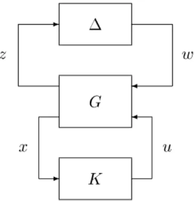
The disturbance

^w

in (1) usually represents uncertainty arising from various locations in the control system. To specify the location and structure of the uncertainty, the robust control paradigm depicted Fig.1 is popular. The system is an uncertainty and

^K

is a state-feedback controller. The system

^G

not only describes a nominal plant, but also includes information about how the uncertainty aects the nominal plant such as geometrical locations and types of nonlinearities where uncertain parameters are present. This uncertainty structure is described by the input map in

^G

at

^w

and the output map in

^G

at

^z

. The principal problem of robust control for the uncertain system is to construct a controller

K

achieving global robust stability:

Global robust stability

If the closed-loop system is globally stable in the presence of every belonging to a given family of admissible uncertainties, the system is said to be globally robustly stable.

The structure of the uncertainty denes the set of disturbances

^w

in (1), (2) and (3). It is well known that such a robust control design usually comes at the price of solving a Hamilton-Jacobi partial dierential equation (3) with an appropriate function

^L

. Such a task is generally not feasible.

This infeasibility of solving HJ equations motivated the development of the inverse optimality direction in robust nonlinear control [6]. Roughly speaking, an inverse optimal design is an optimal design in which the choice for the function

^L

is left open:

Global inverse optimality

If there exist a function

^L

such that (3) has a positive denite and radially unbounded solution

V

(

^x

) on

^R

ⁿ , then the control

^u

achieving minimum of (3) is said to be globally inverse optimal.

Inverse optimality exploits the fact that an HJ equation with a xed function

^L

is only a sucient

condition for achieving robustness. The inverse optimal design seeks a particular solution to an

appropriate class of HJ equations which lead to desired robustness of a system by using

^L

as a

design parameter. It is important to remember that the inverse approach enables us to design robust

controllers without solving HJ equations directly, provided the function

^L

is chosen from an appropriate

class.

(4)

According to Lyapunov's rst method, we can achieve stability robustness in Fig.1 at least locally by using a linearized description of the system. Fortunately, an HJ equation for a linearized system reduces to an algebraic Riccati equation which can be solved easily and eciently. The optimal controller directly guarantees the stability robustness in Fig.1 for linear

^G

and families of including memoryless and dynamic, structured and unstructured uncertainties. Thus, for achieving robustness at least locally, the following property is desirable:

Local optimality

Suppose that a function

^L

is given a priori so that it describes desired stability robustness. If the linearization of a control law

^u

at

^x

= 0 is an optimal control associated a value function which solves the linear version of (3) (i.e., Riccati equation), the control law

^u

is said to be locally optimal.

However, a controller that performs well on a linearized model may drastically reduce the stability region of the actual nonlinear system. Local optimality by itself is not sucient for inherently nonlinear systems.

If maximization with respect to

^w

is dropped in the global inverse optimal design, then global optimality does not necessarily imply global robust stability. For example, consider the following choice for

^L

which is a natural generalization of LQ optimal control:

L

=

^q

(

^x

) +

^r

(

^x

)

^u²^; ^q

(

^x

)

0

^; ^q

(0) = 0

^; ^r

(

^x

)

^>

0

^8x²^R

ⁿ (4) with optimality described by

J

opt = min _u

^Z ¹

0

L

(

^x;^w;^u

)

^dt

subject to

^w

0 (5)

instead of (2). A global inverse optimal controller with respect to (5) may exhibit robustness properties in the sense of stability margins [10], but it generally only guarantees stability robustness with respect to certain types of input uncertainties. In fact, in general the optimal controller does not achieve robustness for the disturbance

^w

as specied in Fig.1. In contrast, for the same function

^L

in (4), global optimality in terms of (2) implies robust stability of the system in Fig.1 because

^J

opt

^< ¹

implies

^x

(

^t

)

^!

0 as

^t ^! ¹

. It is known that robust stabilizability of the system with the family of memoryless uncertainties is equivalent to the existence of a robust control Lyapunov function (rclf). In fact, it has been shown in [6] that every rclf solves an HJ equation associated with the cost functional (2) and the inverse optimal control law is given in terms of the rclf. The inverse optimal control in [6] thus takes robust stability into account. However, the relationship between the global optimality achieved and robust stabilization of the linearized system is not clear. Indeed, in general, the globally inverse optimal control law is not locally optimal.

Another candidate for the function

^L

in (2) for inverse optimal control is as follows:

L

=

^q

(

^x

) +

^r

(

^x

)

^u²^;²^w²^; ^q

(

^x

)

0

^; ^q

(0) = 0

^; ^r

(

^x

)

^>

0

^8x²^R

ⁿ (6)

Because this

^L

is a natural generalization of linear

^H¹

optimal control, it has been shown in [8] that

the associated globally inverse optimal controllers can be locally

^H¹

optimal for a class of nonlinear

systems. However, because of the negative term in

^L

, global inverse optimality does not necessarily

assure global robust stability in the presence of the disturbance

^w

. In [7], a terminal penalty is

(5)

introduced which excludes this possibility of destabilizing inverse optimal controllers:

J

opt = min _u max _w

(

T lim

^!1

"

E

(

^x

(

^T

)) +

^Z

^T

0

q

(

^x

) +

^r²

(

^x

)

^u²^;^r¹

(

^x

)

^w²^dt

# )

(7)

q

(

^x

)

0

^; ^q

(0) = 0

^; ^r¹

(

^x

)

0

^; ^r²

(

^x

)

^>

0

^; ^8x²^R

ⁿ

Here,

^E

is a positive denite radially unbounded function. It was proved in [7] that for a class of input-to-output stabilizable systems, input-to-output stability can be achieved in the presence of input unmodeled uncertainty. However, this type of global stability is guaranteed for a certain class of unstructured input uncertainties which in general does not conform to the location/structure specied in Fig.1. Furthermore, the inverse optimal control in [7] is not guaranteed to be locally optimal.

The purpose of this paper is to develop a backstepping procedure which meets all the three objec- tives simultaneously: global inverse optimality, local optimality, and global robust stability. For this purpose, an appropriate choice of

^L

will given by generalized state-dependent scaling.

3 Denitions

Consider the uncertain nonlinear system described by

: _

^x

=

^A

(

^x

)

^x

+

^B

(

^x

)

^w

+

^G

(

^x

)

^u ^:

(8) where dimensions of signals are

^x

(

^t

)

²^R

ⁿ ,

^u

(

^t

)

²^R¹

,

^w

(

^t

)

²^R

^p . Functions

^A

(

^x

),

^B

(

^x

) and

^G

(

^x

) are assumed to be suciently smooth. We make the following structural assumptions on these matrices.

First, we assume that

^A

,

^B

and

^G

can be written in the form

A

(

^x

)=

2

6

4 a

11

(

^x

)

^a¹²

(

^x

) 0

0

a

21

... ... (

^x

)

^a²²

... ... (

^x

)

^a²³

... ... ... ... ... (

^x

) 0 ... 0 0

a

n

^;1

;

¹

(

^x

)

^a

n

^;1

;

²

(

^x

)

^a

n

^;1

;n (

^x

)

a

n

¹

(

^x

)

^a

n

²

(

^x

)

^a

nn (

^x

)

3

7

5

(9)

B

(

^x

)=

2

6

4 B

11

(

^x

) 0

0

B

21

... (

^x

)

^B²²

... ... 0 (

^x

) ... ...

B

n

¹

(

^x

)

^B

n

²

(

^x

)

^B

nn (

^x

)

3

7

5

;G

(

^x

)=

2

6

4

0... 0

a

n;n

⁺¹

(

^x

)

3

7

5

:

(10)

Each scalar-valued function

^a

ij is required to satisfy

a

ij (

^x

) =

^a

ij (

^x¹^;^x²^;^;^x

i )

^;

1

ⁱ^n;

1

^jⁱ

+ 1 (11)

a

i;i

⁺¹

(

^x¹^;^x²^;^;^x

i )

⁶

= 0

^;

1

ⁱⁿ

(12) for all

^x ²^R

ⁿ . The dimension for the matrix

^B

(

^x

) is

^B

ij (

^x

)

²^R¹

^p

ⁱ

and

^p

=

^P

_ni

⁼¹^p

i ,

^p

i

0. Its dependence on

^x

is

B

ij (

^x

) =

^B

ij (

^x¹^;^x²^;^;^x

i )

^;

1

ⁱ^n;

1

^jⁱ^:

(13)

Denition 1 Given a positive semi-denite, radially unbounded, C

¹

function

^V

(

^x

) and a positive scalar-valued function

^r

(

^x

), the control law

u

(

^x

) =

^;

1

2

^r^;1

(

^L

G

^V

) ^T (14)

is globally inverse optimal with disturbance level

when

(6)

(i) The equilibrium

^x

= 0 of is globally asymptotically stabilized by (14) when

^w

0. (ii) There exist a scalar-valued function

^q

(

^x

) and a

^R

^p

^p -valued function (

^x

) such that

L

Ax

^V

+ 1 4

²^L

^B

^V

^;1

(

^L

B

^V

) ^T

^;

1

4

^L

^G

^V^r^;1

(

^L

G

^V

) ^T +

^q

= 0 (15)

q

(

^x

)

0

^; ^r

(

^x

)

^>

0

^;

(

^x

) = ^T (

^x

)

^>

0

^; ^8x2^R

ⁿ

^:

The control law (14) with a solution to (15) minimizes the worst-case value of the cost functional

J

(

^u;^w

) =

^Z ¹

0 h

q

(

^x

) +

^r

(

^x

)

^u²^;²^w

^T (

^x

)

^wⁱ^dt

(16) subject to the disturbance

^w

over all stabilizing control laws, i.e., min u max w

^2L2^J

(

^u;^w

) is achieved.

The function

^V

(

^x

) is the optimal value function[15, 16]. The disturbance penalty in the cost functional (16) was refereed to as state-dependent weighting in [7]. It has been proved that if (8) is input-to- state stabilizable, then the inverse optimal problem is solvable with respect to (16)[7]. Note that the function

^V

(

^x

) satisfying the Hamilton-Jacobi-Isaacs(HJI) equation (15) is positive denite if

^q

(

^x

)

0 implies

^x

0. In the cost functional (16), since can absorb

, the roll of

is not clear in Denition 1. The meaning of

in connection with robustness will be discussed in Section 7. When

^p

= 0, the inverse optimal control dened in Denition 1 reduces to the inverse optimality without disturbance [6, 10].

We now consider Jacobian linearization of as follows:

_

x

=

^A

l

^x

+

^B

l

^w

l +

^G

l

^u

l (17)

A

l =

^@f

@x

x

⁼⁰

=

^A

(0)

^; ^B

l =

^B

(0)

^; ^G

l =

^G

(0)

^:

(18) We assume that

^Q

l =

^Q

_Tl

^>

0,

^r

l

^>

0 and l = _Tl

^>

0. Then, since (

^A

l

^;^G

l ) is controllable by our assumptions on

^A

(

^x

) and

^G

(

^x

), there exists a positive number

such that

A

Tl

^P

l +

^P

l

^A

l +

^P

l

1

2

B

l

^;1^B

_Tl

^;G

l

^r^;1

l

^G

Tl

^P

l +

^Q

l =0 (19) has a unique solution

^P

l =

^P

_Tl

^>

0 for

^>

and the control law

u

l =

^;r

_l

^;1^G

_Tl

^P

l

^x

(20)

stabilizes the linear system (17). The control law (20) with the solution

^P

l

^>

0 to the Riccati equation (19) achieves min u

^l

max w

^l^2L²^J

l (

^u

l

^;^w

l ) for the cost functional

J

l (

^u

l

^;^w

l ) =

^Z ¹

0 h

x

T

Q

l

^x

+

^r

l

^u²

l

^;²^w

Tl l

^w

l

i

dt

(21)

over all stabilizing control laws

^u

l . Here,

^V

l (

^x

) =

^x

^T

^P

l

^x

is the optimal value function.

Denition 2 Suppose that

^Q

l =

^Q

_Tl

^>

0,

^r

l

^>

0 and l = _Tl

^>

0 are given and

is chosen as

>

. The control law (14) is said to be locally optimal and globally inverse optimal with disturbance level

if

(i) the control (14) is globally inverse optimal with disturbance level

.

(7)

(ii) the Jacobian linearized control law

u

=

^;

1

2

^r^;1

(0)

^G

^T (0)

^@²^V

@x 2

x

⁼⁰

x

(22)

stabilizes the linear system (17) and achieves min u max w

^2L2^J

l (

^u;^w

).

(iii)

^q

(

^x

)

0,

^r

(

^x

)

^>

0 and (

^x

) = ^T (

^x

)

^>

0 satisfy 2

^Q

l =

^@²^q

(

^x

)

@x 2

x

⁼⁰

; r

l =

^r

(0)

^;

l = (0) (23)

If (

^x

) is restricted to an identity matrix for all

^x ² ^R

ⁿ , the above denition reduces to the local optimality and global inverse optimality dened in [8].

Without loss of generality, l = (0) is assumed to be a diagonal matrix throughout this paper.

In fact, we can always replace any l

^>

0 with an identity matrix as follows. Decompose l into l =

^W

^T

^W

with a lower triangular matrix

^W

by using the Cholesky factorization. By dening

w

l =

^W^w

l , the

^w

l -term in (21) becomes

²^w

_Tl l

^w

l =

²^w

_Tl

^w

l . Since

^W

is lower triangular,

^B

(

^x

)

^W^;1

is again in the block lower triangular form of (10). Consider the inverse optimal problem of

J

(

^u;^w

) =

^Z ¹

0 h

q

(

^x

) +

^r

(

^x

)

^u²^;²^w

^T (

^x

)

^wⁱ^dt

(24) for the system in which

^B

(

^x

)

^w

of is replaced with

^B

(

^x

)

^W^;1^w

. This problem is the same as the inverse optimal dened with (16) for the original system with respect to (

^x

) =

^W

^T (

^x

)

^W

, while in the optimal control with respect to (24), we have (0) =

^W^;

^T (0)

^W^;1

=

^I

p as desired.

4 Global inverse optimality via generalized SD scaling

We now consider the following weighting functions for the cost

^J

in (16):

q

(

^x

) =

^x

^T

^C

^T (

^x

)(

^x

)

^C

(

^x

)

^x

+

^x

^T

^Q

(

^x

)

^x

(25)

r

(

^x

) =

U (

^x

)

^;

(

^x

) = ^T (

^x

) (26) (

^x

)

^>

0

^; ^Q

(

^x

)=

^Q

^T (

^x

)

^>

0

^;

U (

^x

)

^>

0

^;

(

^x

)

^>

0

^; ^8x2^R

ⁿ

The matrix

^C

(

^x

)

²^R

^q

ⁿ is a prescribed function and it is assumed to have the form

C

(

^x

)=

2

6

4 C

11

(

^x

) 0

0

C

21

... (

^x

)

^C²²

... ... 0 (

^x

) ... ...

C

n

¹

(

^x

)

^C

n

²

(

^x

)

^C

nn (

^x

)

3

7

5

;

C

ij (

^x

)=

^C

ij (

^x¹^;^x²^;^;^x

i )

1

ⁱ^n;

1

^jⁱ

(27)

for suciently smooth functions

^C

ij (

^x

)

² ^R

^q

ⁱ¹

,

^q

i

0 and

^q

=

^P

_ni

⁼¹^q

i . The matrices (

^x

) and (

^x

) are parameters to be used for achieving the inverse optimality of Denition 1. The matrices are assumed to consist of scalar-valued functions

i (

^x

) and

i (

^x

),

ⁱ

= 1

^;

2

^;^:^:^:^;ⁿ

with

(

^x

)=block-diag[

¹

(

^x

)

^I

q

¹^;²

(

^x

)

^I

q

ⁿ^;^;

n (

^x

)

^I

q

ⁿ

] (28)

(

^x

)=block-diag[

¹

(

^x

)

^I

p

¹^;²

(

^x

)

^I

q

ⁿ^;^;

n (

^x

)

^I

p

ⁿ

]

^:

(29)

(8)

Here,

^I

q

ⁱ

denotes a

^q

i

^q

i identity matrix. Each

i or

i is a function of

^x

of the form

i (

^x

)=

i (

^x¹^;^x²^{; ;}^x

i )

^;

i (

^x

)=

i (

^x¹^;^x²^{; ;}^x

i )

^;

1

ⁱⁿ

The scalar-valued function

U is also a parameter to be chosen in the inverse optimal design and its dependence on

^x

is

U (

^x

) =

U (

^x¹^;^x²^;^;^x

n )

^:

We assume that

i (

^x

)

^>

0

^;

i (

^x

)

^>

0

^; ^8i;

U (

^x

)

^>

0

^; ^8x²^R

ⁿ

^:

Substituting the above parameters into (16), the cost function

^J

(

^u;^w

) becomes

J

(

^u;^w

) =

^Z ¹

0 h

z

T (

^x

)

^z

+

^x

^T

^Q

(

^x

)

^x^;²^w

^T (

^x

)

^wⁱ^dt

(30) with an augmented system

a :

^x

_ =

^A

(

^x

)

^x

+

^B

(

^x

)

^w

+

^G

(

^x

)

^u

z

=

^C

(

^x

)

^x

+

^Hu ^;

(31)

where

C

(

^x

)=

2

6

4 C

11

(

^x

) 0

0

C

21

... (

^x

)

^C²²

... ... 0 (

^x

) ... ...

C

n

¹

(

^x

)

^C

n

²

(

^x

)

^C

nn (

^x

)

0 0 0 0

3

7

5

; H

=

2

6

4

0 0 0 ...

1

3

7

5

(32)

(

^x

) = block-diag[(

^x

)

^;

U (

^x

)]

^:

(33)

The cost functional (30) can be rewritten as

J

(

^u;^w

) =

^Z ¹

0

"

n

X

i

⁼¹

(

i (

^x

)

^z

_Ti

^z

i

^;²

i (

^x

)

^w

_Ti

^w

i ) +

^x

^T

^Q

(

^x

)

^x

+

U (

^x

)

^u²

#

dt

(34)

where

^w

and

^z

are partitioned as

w

=[

^w

^T

¹^;^;^w

_Tn ] ^T

^; ^w

i

²^R

p

ⁱ; z

=[

^z¹

^T

^;^;^z

_Tn

^;^u

] ^T

^; ^z

i

²^R

q

ⁱ :

When we choose

i =

i for

ⁱ

= 1

^;

2

^;^:^:^:^;ⁿ

in (34), the parameter

i (

^x

) becomes the state-dependent(SD) scaling [12]. Therefore, in this paper, we call ((

^x

)

^;

(

^x

)) the generalized state-dependent scaling for inverse optimal control.

Let

^x^[

k

^]

denote the states

^x¹

through

^x

k .

x

[

k

^]

=

^x¹ ^x² ^x

k

T

We consider a dieomorphism

=

^S

(

^x

)

^x

between

^x²^R

ⁿ and

²^R

ⁿ . Let

^S^;1

(

^x

) denote the inverse map of the dieomorphism and choose

S

;1

(

^x

) =

2

6

4

1 0 0 0

0

s

1

(

^x

) 1 0 0

0

d

21 s

2

(

^x

) 1 0 ... 0

d

31 d

32 s

3

(

^x

) 1 ... 0 ... ... ... ... ... ...

d

n

^;1

;

¹ ^d

n

^;1

;n

^;2 ^s

n

^;1

(

^x

) 1

3

7

5

;

(35)

(9)

where the smooth scalar functions

^s¹

(

^x¹

)

^;^s²

(

^x^[2]

)

^;

,

^s

n

^;1

(

^x^[

n

^;1]

) are to be determined in a recursive manner from

^s¹

through

^s

n

^;1

. Each function

^s

i depends only on the state components

^x¹

through

^x

i . The other scalar constants

^d

ij , 2

ⁱⁿ^;

1, 1

^j ⁱ^;

1, are any real numbers. Then,

^S

(

^x

) is

S

(

^x

) =

2

6

4

1 0 0

0

4

1

1 0

0

4

2 4

2

1 ... ...

... ... ... ... 0

4

n

^;1 ⁴

n

^;1

1

3

7

5

where

⁴

j denotes any function depending only on

^s¹

through

^s

j . This dieomorphism

^S

(

^x

) is the same as the one in [6] and [14] if we take

^d

ij = 0. The time-derivative of

is

_

=

^@S

@x

1 x;

@S

@x

2 x;;

@S

@x

n

^x

_

x

+

^S

(

^x

)_

^x

=

^T

(

^x

)_

^x^:

(36) with a smooth function

^T

(

^x

):

T

(

^x

) =

2

6

4

1 0 0

0

?

1

;

¹

1 0

0

?

2

;

² ^?²

;

²

1 ... ...

... ... ... ... 0

?

n

^;1

;n

^;1 ^?

n

^;1

;n

^;1

1

3

7

5 :

The entries

^?

i;j depend only on the states

^x¹

through

^x

i and the functions

^s¹

through

^s

j and their partial derivatives. We now consider a state-feedback law

u

(

^x

) =

^s

n (

^x^[

_n

^]

)

n (37) where

^s

n is another smooth function yet to be determined. Then, the closed-loop system consisting of (31) and the state-feedback law becomes

cl :

(

_ =

^T^A

^

^S

^ +

^Bw

z

= ^

^C^S

^ (38)

^

S

:=

0

^S^;1

0

^s

n

; ^A

^ := [

^A ^G

]

^; ^C

^ := [

^C ^H

]

^:

Theorem 1 Suppose that

^P

= diag[

^P¹^;^P²^;^;^P

n ] is a constant diagonal matrix and

M

(

^x

):=

2

6

4

^

S

T

^A

^ ^T

^T

^P

+

^P^T^A

^

^S

^

^;1^P^TB ^S

^ ^T

^C

^ ^T

;1

B

T

P ;

0 ^

^C^S

^ 0

^;

3

7

5

<

0 (39)

P >

0 (40)

are satised for all

^x² ^R

ⁿ , Then, the nonlinear system is globally asymptotically stabilized by the state-feedback law

^u

=

^s

n

n and

J

(

^u;^w;^T

) =

^Z

^T

0 h

z

T (

^x

)

^z

+

^x

^T

^Q

(

^x

)

^x^;²^w

^T (

^x

)

^wⁱ^dt

V

(

^x

(0))

^;^V

(

^x

(

^T

)) (41)

Generalized State-Dependent Scaling for Local Optimality, Global Inverse Optimality,

ISSN 1344-8803, CSSE-7 January 31, 2000