1 明星大学理工学部総合理工学科機械工学系 常勤教授 空気力学 Meisei University, Mechanical Engineering, Professor by contract, Aerodynamics 2 明星大学理工学部総合理工学科機械工学系 教授 流体力学 Meisei University, Mechanical Engineering, Professor, Fluid Dynamics
【研究論文】
層流旋回浮力流れの解析モデル
森 下 悦 生
1熊 谷 一 郎
2Mathematical Model of Laminar Whirling Buoyant Flow Etsuo MORISHITA1, Ichiro KUMAGAI2
In this paper, the laminar whirling buoyant flow in a rotating vertical pipe with an axial line heat source of constant temperature is solved analytically. While there are numerous detailed experimental and numerical investigations of the thermal spiral flows, the analytical solution is an approximate model of a laminar fire whirl. In laboratory experiments, the thermal whirling flow is generated by a point heat source with a pair of stationary vertical eccentric half pipes; instead, a constant circumferential pipe wall velocity is given as one of the boundary conditions in this model. The Boussinesq approximation is applied for the buoyancy. The Navier–
Stokes equations in cylindrical coordinates are simplified by neglecting the inertia terms. The derivatives along the vertical axis vanish based on the assumption of fully developed flow. The radial velocity component is also zero owing to the same assumption.
The quantities along the circumferential direction remain unchanged. The buoyancy velocity distribution is similar to that of the Hagen–Poiseuille flow with an extra logarithmic term due to the radial temperature distribution. The tangential whirl velocity is independently obtained as a potential circulation. The natural convective heat transfer formula is obtained, and the Grashof number becomes a linear function of the Reynolds number, where the radius of the line heat source is a parameter.
キーワード:管内流, 循環, 自然対流, 浮力, 火炎旋風
Keywords:pipe flow, circulation, natural convection, buoyancy, fire whirl
1. Introduction
The study of fire whirls is important for not only understanding the natural phenomena but also preventing such disasters (1)-(7). A laboratory-scale fire whirl can be easily created with two transparent plastic half pipes which are slightly off-center (i.e.
eccentric) (8). Alcohol can be used as the fuel at the bottom of the vertical half pipes, and the resulting flame to rises because of buoyancy. Combustion is very stable without the half pipes. When the flame is surrounded by a pair of eccentric vertical half pipes, a small fire whirl develops owing to the circulation from the vertical slits between the two pipes.
Another interesting experiment is a smoke whirl with a mosquito coil, as shown in Fig. 1(9), (10). At the very beginning, smoke rises vertically yet fluctuates. After a while, the smoke follows a spiral flow, which is equivalent to the fire whirl. In this experiment, the flow can be visualized by a light sheet. A horizontal cross section is visualized and the smoke circulation is visible; the vertical plane is also visualized.
In particular, this small laminar smoke whirl from the mosquito coil can be modelled mathematically as buoyant pipe flow with a line heat source of constant temperature along the vertical axis.
Side view Cross section Fig.1 Whirling smoke flow from a mosquito coil (transparent half pipe diameter/height/offset:100 mm/500 mm/10 mm)
Instead of the two side slits in the experiment, a constant circumferential wall velocity is used. The Boussinesq approximation is applied for the buoyancy. The convective terms should be negligible in the spiral smoke flow, so the Navier–Stokes equations in the cylindrical coordinate are simplified accordingly.
The vertical and the radial derivatives vanish owing to the assumption of fully developed flow. The tangential flow derivatives also vanish.
2. Governing Equations and Solutions
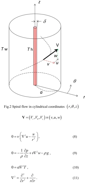
Figure 2 shows the present equivalent flow model for approximating the smoke whirl shown in Fig. 1. The circulation from the side slits is replaced by the artificial tangential velocity of the pipe wall to simplify the flow model. The line heat source at constant temperature along the vertical axis models the heated smoke, and this isothermal region is assumed to be gaseous.
The governing equations for an incompressible flow in cylindrical coordinates of Fig. 2 are given as follows:
rv u w 0 r r r z
, (1)
2
2
2 2
1 2
v v v u v w v u
t r r z r
p v v u
r r r
, (2)
2
2 2
1 2
u u u u u uv
v w
t r r z r
p u v
r u r r
, (3)
1 2
w v w u w w w
t r r z
p w g
z
, (4)
T T u T T 2
v w T
t r r z
, (5)
where r is the radial coordinate, is the circumferential coordinate, zis the vertical coordinate, vis the radial velocity,
uis the circumferential velocity, wis the vertical velocity, tis time, pis pressure, is the density of air, is the kinematic viscosity, is the dynamic viscosity, g is gravitational acceleration, Tis temperature, is the thermal diffusivity, Th is the heat source temperature, Twis the wall temperature, is the line heat source radius and
2 2 2
2
2 2 2 2
r r r r z
. (6)
The following approximations are applied:
0 v , 0
t
, 0
, 0, p const
z z
.
The governing equations without the convective terms become
2 1
u p
r r
(7)
Fig.2 Spiral flow in cylindrical coordinates r, , z
V V Vr, , z v u w, ,
V
2
0 u2
u r
, (8)
1 2
0 p w g
z
, (9)
0 2T, (10)
2 2
r2 r r
. (11)
Combining Eqs. (8) and (11), the tangential velocity is found to be inversely proportional to the radial coordinate:
u A
r . (12) From Eq. (7), we obtain
ref
2
2
2 A p p
r
. (13)
where pref is the reference pressure. The pressure coefficient is defined as
2
ref ref
p
2 ref
1 1
1 2
p p r
C u r
. (14)
The energy equation, i.e. the radial heat conduction equation, becomes
z
r
V
v u
w T h
T w
a
2
2 0
T T T
r r r r r r r
, (15)
with boundary conditions
TTh at r 0 r , (16)
T T wat ra ra. (17) From Eqs. (15)–(17), the temperature is given by
w
h w ref
ln ln
r
T T T a
T T T
a
. (18)
The Boussinesq approximation is given by
0 0
0
1 1 T
, (19)
where is the thermal expansion coefficient and 0denotes the ambient density. From Eq. (19), Eq. (9) becomes an ordinary differential equation:
w
0 P d dw
r g T T
z rdr dr
, (20)
where 0and the excess pressure Pis defined as
P p gz. (21)
The boundary conditions for Eq. (20) are dw 0
dr at r0, (22) 0
w at ra. (23) Equation (20) can be solved analytically with the temperature distribution of Eq. (18) as follows:
2 2
2 2
ref 2
1 1 1
4
1 1 ln
ln 4
P r
w a
z a
g T r r r
a a a a
a
. (24)
The first term in the right hand side of Eq. (24) corresponds to the Hagen–Poiseuille flow; the second term, whose derivation implicitly assumes a, represents the thermally driven flow.
In this simplified mathematical model, the radial velocity component is zero, and the tangential velocity is independently given by Eq. (12).
The average velocity waveis derived from the volume flow rate Qas follows:
2 2
ref
ave 2 5 7
3
2 2 ln 1
g T
Q d dP d
w a dz
a
, (25)
whered2a is the diameter. The dimensionless form of Eq.
(25) is
6 7
1 3
2 2 ln 1
dP Gr
Re dz
a
, (26)
where the Grashof and the Reynolds numbers are defined together with the normalized pressure and coordinate as follows:
3 ref
2
Gr T gd
, (27)
w dave
Re
, (28)
1 2
2 P P
d
, (29)
z z
d . (30)
The first term in the right-hand side of Eq. (26) corresponds to the different form of the pipe friction coefficient 64 /Reowing to the different reference velocity.
From Eqs. (25) and (26), the flow condition Q0wave 0
is given by 3 2 ln 1
dP Gr
dz
a
. (31)
At the critical condition Q w ave 0, we obtain
crirical
3 0
2 ln 1
dP Gr
dz
a
. (32)
The velocity distribution at dP dz/ criticalbecomes
critical 5
5
2 2
1 1 3 2
1 1 3
3 2 2 ln 1
1 4 ln
w dP d dz
w Gr d
a
r r r
a a a
. (33)
Equation (33) represents an updraft in the core with descending airflow in the outer region. If the adverse pressure gradient is greater thandP dz/ critical , the flow rateQ is negative and the buoyancy effect is hampered by the pressure, although this situation is rather mathematical.
In the smoke whirl experiment shown in Fig. 1, effectively no external pressure gradient exists: dP dz/ 0.
For a purely thermally driven flow with dP dz/ 0 in Eq.(24), we obtain
ave 7
3 2 ln 1 w Gr
d a
, (34)
3
max 4 ave
1 2
2 ln 1 3
w Gr w
d a
, (35)
2 2
max
1 ln
w r r r
w a a a
, (36)
7
3 2 ln 1 Re Gr
a
, (37)
where wmax is the maximum velocity along the vertical axis
/ 0
r a . Equation (37) is derived from Eq. (34), and it indicates that the thermally induced flow is proportional to both the temperature difference and the size of the heated core.
3. Computational Results
Figure 3 shows the thermally driven buoyant flow, Eq. (36), together with the Hagen–Poiseuille flow. Figure 4 shows the temperature distribution, Eq. (18). The temperature is assumed to be constant as T Tw for0 r . The constant temperature core is assumed to be fluidic. Equation (37) is shown in Fig. 5 with
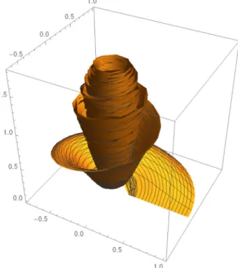
the heated core ratio /a as a parameter. Figures 6 shows the spiral path lines forr a/ 0.2,0.5 and1 , and the same vortex stream surface is shown in Fig.7, where
, max 2 2
1 ln
z t r w t w t r r r
a a a a a a
, (38)
max 2
max
, 1
A t
w t
ut r A
t r r r aw a r
a
, (39)
andv0. The pitch of the spiral is given by
2 2
max
2 2
max
2 2
max
1 ln
1 ln
1 ln
r r r
w a a a
dz w
rd u u
r r r
w a a a
A r
aw r r r r
A a a a a
. (40)
In Fig.6, two non-dimensional values, i.e. circulation Aand time t , are defined as follows:
max
A A
aw , (41)
w tmax
t a . (42)
From Eq. (40), the pitch of the spiral takes the maximum value at 0.492
r
a .
Fig. 3 Buoyant and Hagen–Poiseuille flows 0
0.5 1
0 0.5 1
buoyancy flow
Poisueille flow
r/a
w/ wmax
Fig. 4 Temperature distribution
Fig. 5 Buoyant flow with a line heat source size /a
Fig. 6 Spiral path line (r a/ 0.2,0.5,1.0, A1, 0 t 2) (11)
Fig. 7 Spiral stream surface (r a/ 0.2,0.5,1.0, A1, 0 t 2) (11)
4. Concluding Remarks
A fire whirl can be generated in the lab by surrounding a flame with a pair of eccentric half pipes. An alcohol lamp or a mosquito coil is placed in the bottom of the pipe in the experiment. From the experimental flow visualization, a simple mathematical model for the laminar spiral buoyant flow was proposed. The model assumes a fully developed flow with an axial line heat source at constant temperature and pipe wall rotation instead of the circulation due to the slits of the eccentric half pipes. The radial velocity component is zero and the circumferential velocity component has the same form as that of a potential-free vortex, i.e. inversely proportional to the radial coordinate. The circulation is proportional to the pipe rotational speed. The radial temperature is determined from the heat conduction equation. The thermally driven vertical flow is obtained in a closed analytical form from the temperature solution with the Boussinesq approximation. The thermally driven flow has a similar velocity distribution to that of the Hagen–Poiseuille flow with an extra logarithmic term due to the temperature distribution.
The analytical solution of the spiral flow was visualized, and the pitch of the spiral reaches its maximum near the midpoint between the pipe wall and the axis. The radial heat transfer to the pipe wall is obtained, and the Grashof number is proportional to the Reynolds number.
0 0.5 1
0 0.5 1
delta/a=0.01 delta/a=0.05 delta/a=0.1
r/a
T/Tref
0.001 0.01 0.1 1 10 100
1 10 100 1000 10000
delta/a=0.1 delta/a=0.05 delta/a=0.01
Gr
Re
0.5
0.0
0.5
1.0 0.5
0.0 0.5
1.0
0.0 0.5 1.0 1.5
Acknowledgements
We would like to thank Editage (www.editage.com) for English language editing.
References
(1) K. Yamashita, “Occurrence of Fire Whirls around Multiple Fires in Cross Wind (in Japanese)”, Japanese Journal of Multiphase Flow, Vol. 9, No. 2 pp.
105–115(1995)
(2) S. Komurasaki, T. Kawamura, and K. Kuwahara, “Vortex Breakdown in Thermal Convection by Rotating High-Temperature Heat Source (in Japanese)”, RIMS Kôkyûroku, Mathematical Aspects of Complex Fluids, (O. Sano Eds.), Vol. 1081, pp. 180-191(1999)
(3) K. Satoh and K.T. Yang, “Study of Fire Whirl (in Japanese)”, Nagare, Vol.
19, No. 2 pp. 81–87(200)
(4) K. Kuwana, S. Morishita, R. Dobashi and G. Kushida, “Theoretical and Numerical Study on Flame Height of Axisymmetric Laboratory-Scale Fire Whirls (in Japanese)”, Journal of the Combustion Society of Japan, Vol. 51, No. 155 pp. 56–62(2009)
(5) M. Shinohara and S. Matsushima, “Experimental Study of Generation Mechanism of Stationary Fire Whirls Just Downwind of a Flame (in Japanese)”, Nagare, Vol. 33, No. 6, pp. 503–507(2014)
(6) H. Onishi and K. Kuwana, “Flow around a Fire Whirl (in Japanese)”, Journal of the Combustion Society of Japan, Vol. 58, No. 185 pp. 167–
171(2016)
(7) S. Harada, M. Mizuno and G. Kushida, “Effects of Flame Base Condition on Fire Whirl (in Japanese)”, Proc. JSME Tokai Branch 65th Conference, No.163-1. https://doi.org/10.1299/jsmetokai.2016.65._525-1(2016) (8) R. N. Meroney, “Fire Whirls and Building Aerodynamics”,
www.engr.colostate.edu/~meroney/projects/MERFWB.pdf.
(9) K. Onodera, “Fire Whirl with Two Half Pipes (in Japanese)”, Graduate Thesis, Meisei University, Feb.(2018)
(10) E. Morishita, I. Kumagai, K. Onodera, R. Kubota, Y. Moriyama and T.
Yamazaki, “A Mathematical Model for a Laminar Spiral Flow to Approximate Fire Whirl”, O3.40, ECT2018 :The Tenth International Conference on Engineering Computational Technology, Sitges, Barcelona, 4-6 Sept. (2018)
(11) Wolfram Research, Inc., Mathematica, Ver. 11.3, Champaign, IL (2018)