5.#L2#Data#Processing##
and#Product#Status
Makoto&Suzuki*2&
&Chihiro&Mitsuda*1,&Takuki&Sano*2,&Naohiro&&Manago*3,&&
Eriko&Nishimoto*2,4,&Yoko&Naito*4,&Chikako&Takahashi*1,&&
Koji&Imai*5,&Masato&Shiotani*4&
&&&&&&&&&&&&&&&&&*1:&Fujitsu&FIP&,&*2:&ISAS/JAXA,&*3:&Chiba&Univ.,&*4:&Kyoto&Univ.,&&*5:&TOME&R&D&
5.0&Outline
• Design and development before launch"
– Were the L2 related activities adequate or not ? Well designed ? Within schedule ? Acceptable processing speed ? Well-prepared for on orbit operation ? Easy to improve ? Well documented and published ? "
– Subjects"
• Sensitivity study, and design study"
• Forward model: Precision and Accuracy. "
• Retrieval: Setting, A priori"
• Spectroscopy"
• L2 Improvement After The Launch"
– Was the L2 system operated and improved appropriately, on subjects, schedule ?!
– Subjects"
• L2: retrieval setting, a priori, retrieval altitude, Tikhonov Regularization"
• L1B: AOS characteristics, Frequency Calibration, Non-linearity, Pointing knowledge, data ßags"
• Spectroscopy: Spectroscopy review using SMILES data, O3 and O3 isotope laboratory measurements"
• Remaining L2 Issue"
– Are the plan for the L2 improvements adequate ?!
– Subjects for future improvements"
• L1B: Non-linearity"
• L2 v3.0: a priori modiÞcation, Tikhonov regularization to all (as many as possible) species"
• L2 v3.X"
– Baseline Þtting for unexpected AOS characteristics"
– Non-Voigt line-shape calculation"
• Spectroscopy: Ganmmaair, n, pressure shift, Non-Voigt line shape."
• Overall"
– Are the L2 related activities performed adequately as the space agency and the science institute ? Are the L2 related scientiÞc results published timely ? 92
This document is provided by JAXA.
5. Outline
• 5.1 !Design and development before launch!
• 5.2 !L2 Improvement After The Launch!
• 5.3!Remaining L2 Issue!
• 5.4!Summary!
– Are the L2 related activities performed adequately as the space agency and the science institute ?!
– Are the L2 related scientiÞc results published timely ?
5.1 Design and development before launch
• Were the L2 related activities adequate or not ? ! – Well designed ? !
– Within schedule ? (Schedule management, Budget, Man power/Personel)!
– Acceptable processing speed ? (Algorithm, mathematics, CPU)!
– Well-prepared for on orbit operation ? ! – Easy to improve ? !
– Well documented and published ? "
• Subjects!
– Sensitivity study and design study!
– Forward model: Precision and Accuracy. ! – Retrieval: Setting, A priori!
– Spectroscopy!
93 93 Report of SMILES Science Evaluation Panel
This document is provided by JAXA.
L2 Algorithm
• Overall requirements described in SMILES Mission Plan (2002)!
• Sensitivity study and algorithm design (2006-2009)!
• Pre-launch L2 system!
• Improvement after the launch!
• Remaining Issues
Characteristics speciÞed in SMILES Mission Plan
• Detail atmospheric and instrument forward model was required.!
– Random noise in spectra, < 0.5K (0.5 s integration)!
• 0.01 K atmospheric forward model precision.!
– Antenna pattern (Mission Plan, 3.2.4.2) !
• Antenna pattern must be considered.!
– Pointing knowledge (relative) (Mission Plan, 3.2.6.2)!
• 0.0015° or 60 m (1sigma), which was found to be performance limiting factor,!
– Sideband Separation (Mission Plan, 3.3.2.2)!
– Acousto-optic Spectrometer, Frequency Characteristics (Mission Plan, 3.3.3.1)!
– Frequency Calibration (Mission Plan 3.3.3.2)!
• as better as 30 kHz!
94
This document is provided by JAXA.
Mission Plan: Antenna Pattern
-60 -50 -40 -30 -20 -10 0
Normalized gain [dB]
-0.8 -0.6 -0.4 -0.2 0.0 0.2 0.4 0.6 0.8
Antenna elevation angle [deg]
Calculated cut pattern (Az=0) Model cut pattern Pvert(El) of pattern model Peff(El) of pattern model
Figure 3.18E↵ective antenna response pattern.
will be collected and integrated in each unit of the output data. Therefore, the e↵ective response patternPef f(El) is calculated by averagingPvert(El) for six consecutive altitudes as the following:
Pef f(El) =1 6
j=5X j=0
Pvert(El+ (j 2.5)∆El), (3.7) where ∆Elis a unit stepping angle of the SMILES antenna, 0.009375 , which is driven by the Antenna Drive Electronics (ADE).
Figure 3.18 shows the vertical and the e↵ective antenna responses for the pattern model in comparison with cut-responses atAz= 0 for the designed pattern and the model pattern.
All patterns are normalized by each antenna gain. The result shows the sidelobe levels of the vertical and the e↵ective antenna response pattern are approximately 9 dB higher than those of the cut response pattern. It means that SMILES has a higher sensitivity to the atmospheric emissions at adjacent altitudes than expected simply from the vertical cut response pattern.
The HPBW of the vertical response pattern is similar to that of the cut response pattern of the model. They are 0.080 . The e↵ective beam size is 0.090 in HPBW, which is 12 % larger than that for the cut response pattern of the model.
3.2.4.3 Beam Efficiency
In the SMILES antenna specification, the FOV beam efficiency is defined by the ratio of the power radiated into an elliptical cone with a flare-angle of 2.5-time HPBW to the total power radiated by a feed horn. The feed horn adopted for SMILES is a so-called
“back-to-back horn,” which is placed at the interface point between the SMILES antenna and the Ambient Temperature Optics (AOPT). It is a circular corrugated waveguide with
54
Mission Plan: Image band rejection
characteristics (left), and contribution of image band to Band C observation (right)
oscillator (SLO) to both LSB (SIS-MIX-1) and USB (SIS-MIX-2) mixers for frequency down-conversion.
The sideband separation characteristics of the modified Martin-Puplett interferometer are determined by the grid-mirror spacings,d1andd2, of two FSPs. In the design of the SMILES submillimeter-wave opticas, a combination of the spacings,d1= 1.545 mm and d2= 1.572 mm, is adopted as a reasonable choise by which we can achieve image rejection better than 15 dB both for LSB and USB of SMILES observation bands while keeping the di↵erence in local-signal power couplings to USB and LSB mixers less than 0.5 dB. The pass-band transmission and image rejection characteristics calculated around the SMILES obeservation bands by an exact theory for the two FSP combination are shown by red symbols in Fig. 3.28. Although the exact theoretical calculations are rather involved, the transmission and rejection characteristics around the SMILES observation bands are found to be well approximated by simple functions describing power coupling coefficients for the SIS mixer-ito the ANT port,Ki,a, and to the CST port,Ki,c, given by
Ki,j(f) =1 +↵2+ 2↵cos(m⇡ff0)
4 (i= 1 or 2, j=aorc). (3.17) A nonlinear least-squares fitting gave an exellent fit of (3.17) to the exact theoretical calculation as shown in Fig. 3.28 with the values of parameters,m,f0and↵, listed in the
-0.4 -0.35 -0.3 -0.25 -0.2 -0.15 -0.1 -0.05 0
623 623.5 624 624.5 625 625.5 626 626.5
Transmission [dB]
Frequency [GHz]
Exact Calculation Least-Squares Fit (m=24, f0=624.624 GHz, a=-0.973366) Proposed Specification (m=24, f0=624.65 GHz, a=0.94)
-0.4 -0.35 -0.3 -0.25 -0.2 -0.15 -0.1 -0.05 0
647.5 648 648.5 649 649.5 650 650.5 651
Transmission [dB]
Frequency [GHz]
Exact Calculation Least-Squares Fit (m=28, f0=648.954 GHz, a=0.973846) Proposed Specification (m=28, f0=648.95 GHz, a=0.94)
(a) Transmission Characteristics in LSB. (b) Transmission characteristics in USB.
-45 -40 -35 -30 -25 -20 -15
623 623.5 624 624.5 625 625.5 626 626.5
Transmission [dB]
Frequency [GHz]
Exact Calculation Least-Squares Fit (m=24, f0=624.65 GHz, a=-0.9843) Proposed Specification (m=24, f0=624.65 GHz, a=-0.94)
-45 -40 -35 -30 -25 -20 -15
647.5 648 648.5 649 649.5 650 650.5 651
Transmission [dB]
Frequency [GHz]
Exact Calculation Least-Squares Fit (m=28, f0=648.944 GHz, a=-0.983511) Proposed Specification (m=28, f0=648.95 GHz, a=-0.94)
(c) Image rejection characteristics in LSB. (d) Image rejection characteristics in USB.
Figure 3.28Coupling coefficientKijfor signal transmission and image rejection of the SSB filter designed for SMILES. +: Exact theretical calculation for SSB filter; green curves: least-squares fit to the exact calculation; blue curves: simplified model for SSB characteristics of SMILES optics.
65
0.0001 0.001 0.01 0.1 1 10 100
625.12 625.32
625.52 625.72
625.92 626.12
626.32
11 11.2 11.4 11.6 11.8 12 12.2
Brightness Temperature [K]
RF Frequency [GHz]
IF Frequency [GHz]
O3
O3(v2)O3(v2) O3
H35Cl
O3 HO2
O3(v3) O3
h = 16 km h = 30 km h = 50 km
Figure 3.30The e↵ect of the image contributions in Band-B.
0.0001 0.001 0.01 0.1 1 10 100
649.12 649.32 649.52 649.72 649.92 650.12 650.32
11.8 12 12.2 12.4 12.6 12.8 13
Brightness Temperature [K]
RF Frequency [GHz]
IF Frequency [GHz]
ClO
O3 O3 HO2
O3-isotopes O3 + BrO h = 16 km h = 30 km h = 50 km
Figure 3.31The e↵ect of the image contributions in Band-C.
67
95 95 Report of SMILES Science Evaluation Panel
This document is provided by JAXA.
Mission Plan: Characteristics of Acousto- Optics Spectrometer (left) and Spectral
Calibration Accuracy (right)
Figure 3.33Frequency response function of the SMILES/AOS. The typical resolution bandwidth is 1.35 MHz.
snap shot spectrum will be approximately 0.5 K.
3.3.3.2 Frequency Calibration
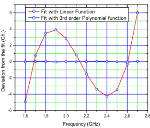
Frequency calibration of the spectrometer will be accomplished by using a frequency reference with the absolute accuracy of about 10 kHz over the whole mission life. It is installed in the IFA section, generating a series of carrier signals with an interval of 100 MHz. The output of this comb generator will be injected to the AOS once in every scan of the antenna (53 seconds). Peak positions of each picket are derived against channel numbers, and the relation between frequency and channel number will be established by a polynomial fitting. Residuals of such fitting will be typically less than 30 kHz as shown in the Figure 3.34, which gives the error in frequency of the AOS spectra.
3.3.3.3 Noise Dynamic Range
Radio signal is converted to optical one in the AOS, and it is detected by a CCD array. The read-out voltages, or the number of collected charges in each cell of the CCD array, should be proportional to the input RF power levels, but they are usually modified by several additional factors in reality. The variance of the original RF noise at CCD is expressed by the following well-known expression:
NRF2 = Q2
B·t, (3.18)
whereQ,B, andtrepresent the number of collected charges at CCD, noise band-width, and the integration time for collecting charges, respectively. Potential contributors to
69
Figure 3.34Residuals from the frequency fit with comb generator. 1 Ch. corresponds to approximately 0.8 MHz.
additional noise are photon shot noise, CCD dark noise, quantization noise, and detection circuit noise:
Nadd2 =Nphoton2 +NCCD2 +NAD2 +NDetection circuit2 . (3.19) The read-out noise of the AOS is the sum of the RF noise and the additional ones:
Nread out2 =NRF2 +Nadd2 . (3.20)
The relative weight of the additional noise will increase as the RF power decreases. So if a criterion is settled so that the noise variance ratioNread out2 /NRF2 to be less than 1.21, then we can define a range of RF power levels, for which the additional noise is less than 10%. We call this the “noise dynamic range” of the AOS. As far as the observed spectra lie within the noise dynamic range, the increase of the system noise due to the AOS can be negligible.
Alternatively, we can calculate an increase of noise at a given signal level. Its coefficient is a function of the signal level, and expressed asf(D), whereD=Qsat/Q, and
Tsysef f=Tsysorg·f(D), (3.21) f(D) can be calculated with the AOS instrumental parameters:
f(D) = vu ut1 +B·t
Qsat·D+B·t q20+qef f2 Q2sat
+ 1
22n·12
!
·D2, (3.22)
where,q0,Qsat,n, andqef fare dark current noise, amount of the saturation charge, quantization bit of the A/D converter, and equivalent amount of charge of the detection
70
Sensitivity Analysis and Algorithm Study
• Sensitivity analysis and Algorithm studies have been conducted JAXA/
ISAS during FY2006-FY2008 (Mar.
2009).!
• Forward Model, Inversion, and A Priori have been studied.
96
This document is provided by JAXA.
Results of Prelaunch Sensitivity Analysis.
0.01 K forward model precision and Instrument Characteristics affect retrieval are considered as much as possible.
0 10 20 30 40 50 60 70
O3 HCl ClO O3-18(a) O3-17(a) CH3CN HO2 HOCl * HNO3 * BrO * Temp.
Altitude [km]
Error < 20 %
Error < 5 % Error < 50 %
1-scan 1-scan1-scan 30-scan
30-scan
30-scan
30-scan
30-scan
30-scan
30-scan
30-scan
30-scan
30-scan Error < 2K
Error < 2 %
O3 HCl ClO* 18OOO 17OOO CH3CN HO2 HOCl HNO3 BrO Temp.
Figure 1.4Altitude coverage of the JEM/SMILES data estimated from preliminary re- sults of simulation studies assuming 0 N standard profile for each molecular species except for ClO for which the standard profile for polar region is assumed. Refer to Chapter 4 for more details.
the equatorial and in the northern high-latitude regions. SMILES data will enable us to investigate the chlorine and bromine chemistry and the HOx chemistry around the polar vortex region and over the equatorial and mid-latitude regions. The SMILES mission also provides a database for ozone variations in time and position around the upper troposphere and lower stratosphere (UT/LS). SMILES’ wide-band and high-resolution spectroscopic data also enables us to investigate the isotopic compositions of ozone. The enrichment of rare isotopes in altitude distribution is reported and expected to reflect some unknown atmospheric processes. Chapter 2 will describe SMILES scientific objectives in detail.
1.4 Overview of the JEM/SMILES Mission
1.4.1 The ISS, JEM, and Measurement Coverage of SMILES
Figures 1.5 and 1.6 show the configurations of the ISS and JEM, respectively. JEM is attached to the front side of the ISS. Scientific experiments will be conducted both in the Pressurized Module (PM) and on the Exposed Facility (EF). JEM-EF has 10 interface ports to accept experiment payloads, four of which are on the front side of the ISS. The use of the interface ports is shared between Japan and the United States. The AO to which the SMILES proposal was submitted was for the first use of four Japanese interface ports. Maximum envelope specified for a JEM-EF experiment unit is 0.8 m (W)⇥1.0 m (H)⇥1.85 m (L). Maximum allowable mass is 500 kg. Services such as electricity, liquid coolant, and data communications including the Ethernet are to be supplied through the EF interface ports.
The ISS has a circular orbit with an inclination angle of 51.6 . Most scientific experi- ments will be conducted while the ISS is in the inertial flight condition to meet microgravity requirements. It results in a steady decrease in altitude, and re-boosting is needed period- ically. The optimum operational altitude of the ISS and the re-boosting period depends
6
SMILES&Mission&Plan&v2.11&(2002)
ozone is the representative species of the SMILES mission.
The main error budgets are Smoothing error.
Retrieval noise.
Forward model parameter errors.
Insufficient information on the profiles of non- retrieved parameters.
Approximations of the instrument functions.
Incorrect input parameters.
Approximations of the fast algorithm.
The retrieval noise can be evaluated from the covariance of measurements,Sy. In case of radiometer whose spectral channels are almost uncorrelated with each other,Syis a diagonal matrix and each diagonal element, sy, is calculated by
sy¼TsysþTA ffiffiffiffiffiffi Bt
p , (20)
whereTAis the measurement brightness temperature, Tsysis the system noise (500 K),Bis the noise bandwidth (2.5 MHz), andtis the integration time (0.5 s).syis one order smaller than that of existing satellite sensors, and the error of ozone retrieval mainly due to retrieval noise is less than 0.5% at 30 km (Fig. 9). This estimation is based on the standard mid-latitude profile, and the standard deviation of a priori profile is assumed to be 100% for all species. Because of the high sensitivity, the forward model parameter errors cannot be considered to be negligible as compared to the retrieval noise. In some cases, the forward model parameters are the most significant errors.
Since most of the forward model parameter errors are systematic errors, they affect the accuracy of the retrieved profiles. We have studied the technique to reduce these errors and have developed an accurate algorithm on the
basis of these studies. As we have showed in Section 3.3, this effect can be reduced to retrieve all species whose signal is larger than a few kelvins (species in the upper row ofTable 1). The instrument functions have been designed to model the measurements, which have been carried out meticulously for each module of the SMILES on the ground by the hardware team of the SMILES. In the determination of the attitude of the ISS for the antenna beam pattern, the error due to FOV convolution is minimized and assumed to be negligible. Basic studies on the incorrect input parameters such as spectroscopic parameters have been carried out by the University of Bremen. However, further studies have to be carried out after the launch.
Although these calculations increase the computing cost since importance is given to accuracy instead of the computing cost, the computing cost can be reduced by using the fast algorithm given in Section 4.4. The speed of calculation using this algorithm is nearly 10 times higher than that of the normal algorithms such as the line selection algorithm and frequency selection algorithm without degradation of the accuracy. The accuracy of the spectra of the stratospheric minor species is up to 0.01 K (1% of the system noise).
5.3. Algorithm performance and hardware system
The algorithm performance has been tested using a 3.16-GHz Quad-Core Intel Xeon processor. The test was performed using the single-scan data of band A, which requires the longest processing time among the three SMILES bands. In band A, seven molecules (Table 1), temperature, and the offset of the tangent altitude are retrieved simultaneously, while in bands B and C, only four molecules (Table 1) are retrieved simultaneously.
Hence, the processing time of bands B and C is approximately 30% lesser than that of band A. We have
ARTICLE IN PRESS
0 10 20 30 40 50 60 70
0 0.1 0.2 0.3 0.4 0.5 0.6 0.7 0.8 0.9 1
Altitude [km]
Error ratio [-]
HClO3 CH3CN HOCl HNO3 asym18-O3 sym17-O3 asym17-O3 ClO
Fig. 9.Retrieval precision of target species that can be retrieved from single-scan data.
C. Takahashi et al. / Journal of Quantitative Spectroscopy & Radiative Transfer 111 (2010) 160–173 171
Takahashi,&Ochiai,&Suzuki&(2010)
A#priori#accuracy#
10°#la<tude#bin,#monthly#a#priori
on the atmospheric temperature from the oxygen emission lines (Livesey et al., 2006; Wehr et al., 1998). Since there is no oxygen line in the SMILES measurement bands, the atmospheric temperature can be derived from the O3emis- sion line at 625.37 GHz (NASDA/CRL, 2002; Verdes et al., 2002; Baron et al., 2001).Fig. 6shows a comparison of the information content (Rodgers, 1998) of the atmo- spheric temperature for the O3 emission line at 625.37 GHz and for the oxygen emission line at 118 GHz under the same conditions as SMILES. It indicates that the atmospheric temperature can be retrieved by using the O3emission line, although it is not as precise as from the oxygen emission line especially in the upper strato-
sphere. The atmospheric temperature and O3vertical pro- files are unknown quantities to be retrieved. Both of them can be retrieved from the same measurement because of the different frequency dependence of their weighting functions.
Fig. 7shows the effect of the atmospheric temperature uncertainty upon retrieved O3profiles. Each line isrdxicor-
0 10 20 30 40 50 60 70
0.001 0.01 0.1 1 10 100
Altitude[km]
Error [%]
Error at the mid-latitude
Random error -5%5%
-10%10%
-50%50%
0 10 20 30 40 50 60 70
0.001 0.01 0.1 1 10 100
Altitude[km]
Error [%]
Error at the tropics
Random error -5%5%
-10%10%
-50%50%
Fig. 5. Estimations for the influence of priori profiles in O3retrieval (in this case, a priori profiles are same as initial profiles). The solid red line is the random error of O3. The other lines are additional errors between the true profiles of O3and the retrieved profiles of O3that are the final results of the iteration process in the cases where the differences between the a priori profiles and true profiles are ±5%, ±10%, and ±50% (top: mid- latitudes, bottom: tropics). (For interpretation of the references to colour in this figure legend, the reader is referred to the web version of this article.)
0 10 20 30 40 50 60 70
9 10 11 12 13 14 15 16 17
Altitude [km]
Information Content [bits]
Ozone Oxygen
Fig. 6. Information content of O3at 625.37 GHz (red/solid line) and oxygen at 118 GHz (green/dashed line). (For interpretation of the references to colour in this figure legend, the reader is referred to the web version of this article.)
0 10 20 30 40 50 60 70
0.001 0.01 0.1 1 10 100
Altitude [km]
Error [%]
Errors of ozone retrieval
Random error 1K2K 10K5K
Fig. 7. Estimation of the influence of uncertainty of initial and a priori profiles of atmospheric temperature (in this case, we retrieve atmospheric temperature and O3profile simultaneously and the priori profiles of atmospheric temperature are same as initial profiles). Lines are additional errors between the true profiles of O3and the retrieved profiles of O3that are the final results of the iteration process in the cases where the uncertainties of atmospheric temperature are 1 K (red/solid line), 2 K (green/dashed line), 5 K (blue/dotted line) and 10 K (pink/fine-dotted line). (For interpretation of the references to colour in this figure legend, the reader is referred to the web version of this article.)
C. Takahashi et al. / Advances in Space Research 48 (2011) 1076–1085 1081
Takahashi, Suzuki, et al. 2011
97 97 Report of SMILES Science Evaluation Panel
This document is provided by JAXA.
Whole spectra Þtting (instead of step-by-step or window approach) is necessary to achieve 1% O3 precision at 20 km.
Windowing may introduce >10% error at 15 km or below.
reason is that the precision of the retrieved instrument pointing by using of band A (or B) is better than by using band C, and the retrieval result is passed to the retrieval processing of band C.
Our retrieval approach for each band consists of two processes. The first process is the retrieval of the target species in the upper row ofTable 1, atmospheric tempera- ture, atmospheric continuum, and the offset of the instru- ment pointing. These component are retrieved simultaneously. The second process, which is performed after the first processes for the two bands, is the retrieval of the target species in the lower row ofTable 1, which are noisy products. These products are retrieved for each product.
We estimate the availability of the simultaneous retrieval for the first process. Fig. 2 indicates the difference of the incremental error for retrieved ozone between simultaneous (blue line) and sequential retrieval (green line) of ozone and HOCl. The red line is the retrieval precision of ozone, which is the square root of the diagonal elements of S. The simulation setting is that the retrieval altitude step is set to 3 km in 4–70 km region, the measurement tangent altitude step is set to 2 km in 0–80 km region, and the instrument parameters are conformed toTable 2. This simulation is performed on band A using all channels. Here we do not estimate the availability of the channel selection to simplify the retrieval scheme.
The incremental error in ozone retrieval for the simultaneous retrieval is approximately 0.1% in the stratosphere and is almost independent of the a priori.
However, the incremental error in ozone retrieval for the sequential retrieval depends on the assumptions of profiles of other molecules such as HOCl. For the case that the true profile of HOCl is 100% and 200% greater than the a priori, the incremental errors of ozone are approxi- mately 1.0% and 2.0% in the stratosphere, respectively.
Furthermore, the iteration number of the sequential retrieval is larger than that of the simultaneous retrieval.
Since this behavior is same as other molecules in the upper row ofTable 1, we adopt the simultaneous retrieval for the first process.
4. Optimized forward model 4.1. Overview of forward model
The forward model calculates the brightness temperatures under the given atmospheric state and also the Jacobians with respect to temperature, the target species concentration, atmospheric continuum, which mainly comes from H2O, and the offset of the instrument pointing. The forward model carries out the following calculations:
1. ray tracing for the evaluation of the atmospheric state along the limb line-of-sight (LOS) with refraction;
2. absorption coefficient calculation for a predefined frequency grid;
3. radiative transfer calculation of the single-ray bright- ness temperature;
4. Doppler shift calculation from the ISS velocity, the rotational velocity of the earth, and wind velocity;
5. signal convolution with the SMILES antenna FOV considering the inclination of the ISS;
6. summation of both sideband signals according to sideband ratio;
7. convolution of infinite resolution spectrum and the instrument frequency response.
The detailed algorithm is given in the following subsec- tions.
0 10 20 30 40 50 60 70
0.001 0.01 0.1 1 10 100
Altitude [km]
Error Ratio [%]
true:a priori = 2:1 Retrieval error
without HOCl with HOCl
0 10 20 30 40 50 60 70
0.001 0.01 0.1 1 10 100
Altitude [km]
Error Ratio [%]
true:a priori = 3:1 Retrieval error
without HOCl with HOCl
Fig. 2.Simultaneous retrieval of ozone and HOCl. The red (solid) line indicates the retrieval precision in ozone retrieval, the green (dashed) line indicates the incremental error in ozone retrieval without HOCl, and the blue (dotted) line indicates the incremental error in ozone retrieval with HOCl. In all these cases, the true profiles of HOCl are 100% (Right) and 200% (Left) greater than the a priori profile of HOCl. Here, the incremental error is defined as the difference between the true profile and the retrieved profile.
Takahashi,&Ochiai,&Suzuki&(2010)
Wind data should be provided for the retrieval. Or, 100 kHz frequency calibration error gives equal to 50 m/s wind velocity error.
10m/s wind velocity error in the stratosphere and 20 kHz frequency calibration error should be achieved. Meteorological data, GEOS-5, is required.
4.3.1. FOV convolution
The FOV of the antenna can be taken into account in the following manner. The brightness temperature con- volved by the FOV at its central tangent altitude z0, TAðn;z0Þ, is obtained by
TAðn;z0Þ ¼ Zzmax
zmin
¯Pðz;z0Þ Tpðn;zÞdz, (13) where Tpðn;zÞ is a single-ray brightness temperature,
¯Pðz;z0Þis a normalized antenna beam pattern convolved along the horizontal direction,zis the tangent altitude, andzminandzmaxare lower and upper tangent altitudes of field viewed by specified main beam when the antenna is pointing to the tangent altitude ofz0.
It is not improbable that the SMILES antenna scan axis is tilted by 15from the horizon, which is inclination of the ISS, from the normal inclination. Since the antenna beam of the SMILES has a horizontally flattened elliptical pattern,¯Pðz;z0Þdepends on the inclination of the antenna scan axis.Fig. 4shows the incremental error in retrieved ozone due to the inclination of the antenna scan axis. If the antenna scan axis inclines by 15, the incremental error is approximately 1% in the stratosphere, and this value is approximately two times larger than the retrieval precision. Therefore, the effect of the inclination of the antenna scan axis should be taken into consideration in the derivation of¯Pðz;z0Þ. The antenna beam patternPðy˜;c˜Þ is measured on the ground with high accuracy, wherey˜ and c˜ are the polar and azimuthal angles, respectively, with respect to thexyz-axis fixed to the antenna. They- axis of the antenna is the direction of the main beam. The x-axis of the antenna is perpendicular to the plane formed by they-axis and a longer axis of elliptically shaped main reflector, and is aligned with rotating axis of the antenna that is elevation steerable. The z-axis of the antenna completes the right-handed axes and is positive toward zenith.Pðy˜;c˜Þis measured by a phase-retrieval method
[31], which is considered to be effective for measuring and evaluating large-scale submillimeter-wave reflector antennas.
The following equations defineyandf. Those are the polar and azimuthal angles which are exactly the same withy˜ and c˜ when thex-axis of the antenna becomes perpendicular to the vector toward the center of the earth.
y˜¼cos1ðsinycoscsinaþcosycosaÞ, (14) c˜¼tan1 sinysinc
sinycosccosaþcosysina
, (15)
whereais the angle of thex-axis of the antenna from the local horizontal plane at the tangent point. Pðy˜;c˜Þ convolved byy,PðyÞ, is
Pðy;aÞ ¼ Z c2
c1
Pðy˜ðy;c;aÞ;c˜ðy;c;aÞÞ cosydc. (16) By using the pre-calculatedPðy;aÞfor every one degree ofa, the incremental error for ozone retrieval can be reduced to less than 0.001%. Finally, ¯Pðz;z0Þis translated from PðyÞ by ray tracing with refraction in every operation calculation.
4.3.2. Sideband ratio
To separate the two sidebands, the SMILES is equipped with a quasi-optical sideband separator in the submilli- meter range. The sideband separator of the SMILES, which is a modified Martin–Puplett interferometer [32], can reject the image band signal more than 20 dB in the SMILES measurement bands. Even in this rejection ratio, the signal from the image band rises up to approximately 2 K in the lower stratosphere. Since this value is not negligible, the image signal should be calculated in our forward model by using the measured response function.
The transmission function,Kbi;jðn;TÞ, from the antennaðj¼ ANTÞor cold sky terminatorðj¼CSTÞto mixer-iin upper
ARTICLE IN PRESS
0 10 20 30 40 50 60 70
0.0001 0.001 0.01 0.1 1 10 100
Altitude [km]
Incremental Error [%]
Ozone
Retrieval error 5 m/s 10 m/s 50 m/s
Fig. 3.Effect of wind. The red (solid) line indicates the retrieval precision of ozone. The other lines indicate the error due to the difference between the reference profile and the true profile of wind. (The wind velocities for the pink (fine dotted), blue (dotted), and green (dashed) profiles are 50, 10, 5 m/s, respectively. The definition of the incremental error is the same as that in Fig. 2.
C. Takahashi et al. / Journal of Quantitative Spectroscopy & Radiative Transfer 111 (2010) 160–173 166
Takahashi,&Ochiai,&Suzuki&(2010)
98
JAXA Special Publication JAXA-SP-13-008E 98
This document is provided by JAXA.