http://dx.doi.org/10.5670/oceanog.2012.43 COPYRIGHT

CITATION

Alford, M.H., J.B. Mickett, S. Zhang, P. MacCready, Z. Zhao, and J. Newton. 2012. Internal waves on the Washington continental shelf. Oceanography 25(2):66–79, http://dx.doi.org/10.5670/

oceanog.2012.43.

DOI

http://dx.doi.org/10.5670/oceanog.2012.43 COPYRIGHT

This article has been published in Oceanography, Volume 25, Number 2, a quarterly journal of The Oceanography Society. Copyright 2012 by The Oceanography Society. All rights reserved.

USAGE

Permission is granted to copy this article for use in teaching and research. Republication, systematic reproduction, or collective redistribution of any portion of this article by photocopy machine, reposting, or other means is permitted only with the approval of The Oceanography Society. Send all correspondence to: [email protected] or The Oceanography Society, PO Box 1931, Rockville, MD 20849-1931, USA.

O ceanography THE OffICIAl MAGAZINE Of THE OCEANOGRAPHY SOCIETY

DOWNlOADED fROM HTTP://WWW.TOS.ORG/OCEANOGRAPHY

Internal Waves ^{on the}

Washington Continental Shelf

S p e C I a l I S S u e O N I N t e r N a l WaV e S

B y M at t h e W h . a l f O r d , J O h N B . M I C k e t t, S h u a N g Z h a N g , pa r k e r M a C C r e a d y, Z h O N g x I a N g Z h a O , a N d J a N N e W t O N

tOp | r/V Thomas G. Thompson crew and John Mickett of apl/uW preparing Cha Ba for deployment off

the Washington Coast. MIddle | field technician Zoë parsons (uW/apl) and r/V Thompson resident

Oceanography | June 2012 67

Internal Waves ^{on the}

Washington Continental Shelf

Oceanography | June 2012 67

mixing. As such, they are thought to be major players in mixing both the deep and shallow ocean. In coastal environ- ments, they have the potential to trans- port nutrients upward into the euphotic zone and transport heat, momentum, nutrients, pollutants, sediment, and even biota such as larvae. However, their slow propagation speed in shallow depths relative to strong low-frequency currents makes them even more variable and complex than in the deep ocean (e.g., see Nash et al., 2012, in this issue).

The Washington continental shelf (Figure 1), at the northern end of the California current system, is a highly bio- logically productive region that has been the topic of considerable attention of late,

owing to its sensitivity to harmful algal blooms (Horner et al., 1997), hypoxic and anoxic events (Whitney et al., 2008), and ocean acidification (Sabine et al., 2004).

A nitrate-limited system, the Washington shelf region appears to be several times more productive than the Oregon or California shelves. Yet, upwelling winds are weaker and more variable than they are further south (Hickey and Banas, 2003). The reasons for this discrepancy have been hypothesized to be related to the presence of the Juan de Fuca Strait, a massive estuary system linking Puget Sound and the Strait of Georgia, the Juan de Fuca eddy, and the Juan de Fuca submarine canyon (Figure 1; Foreman et al., 2008; MacFadyen and Hickey, 2010). In ways that are not yet fully understood, these three unique aspects of the Washington continental shelf may conspire to boost its productivity (Hickey and Banas, 2008).

Internal waves and mixing, are likely key players in these scenarios for Washington waters, though they have not been the subjects of detailed reports.

On the New England and Oregon conti- nental shelves, internal waves are respon- sible for a great deal of the observed mixing, with high-frequency nonlinear internal waves accounting for about half in each case (MacKinnon and Gregg, 2003a; J. Moum, Oregon State University, pers. comm., 2012). In the case of Oregon, turbulence has been observed to enhance the flux of nitrate to the eupho- tic zone (Avicola et al., 2007). Pineda (1999) demonstrated the potential for nonlinear internal tides to transport invertebrate larvae onto the Southern California continental shelf. Finally, Lucas et al. (2011) inferred lateral nitrate fluxes associated with the internal tide INtrOduCtION

Internal gravity waves, the undersea analogue to surface gravity waves, are ubiquitous in the world ocean. They cause density layers to move vertically as much as hundreds of meters, with horizontal currents up to a meter per second, in the most active regions such as the South China Sea (Alford et al., 2011). Thought to be primarily gener- ated by the wind blowing on the ocean’s surface (leading to “near-inertial waves”) and tidal currents flowing over seafloor bumps (leading to “internal tides”), they can give rise to strongly vertically sheared currents and even sweep denser water above lighter water. Both of these instabilities can lead to turbulence and

aBStr aCt. The low-frequency oceanography of the Washington continental

shelf has been studied in great detail over the last several decades owing in part

to its high productivity but relatively weak upwelling winds compared to other

systems. Interestingly, though many internal wave-resolving measurements have

been made, there have been no reports on the region’s internal wave climate and

the possible feedbacks between internal waves and lower-frequency processes. This

paper reports observations over two summers obtained from a new observing system

of two moorings and a glider on the Washington continental shelf, with a focus on

internal waves and their relationships to lower-frequency currents, stratification,

dissolved oxygen, and nutrient distributions. We observe a rich, variable internal

wave field that appears to be modulated in part by a coastal jet and its response to

the region’s frequent wind reversals. The internal wave spectral level at intermediate

frequencies is consistent with the model spectrum of Levine (2002) developed for

continental shelves. Superimposed on this continuum are (1) a strong but highly

temporally variable semidiurnal internal tide field and (2) an energetic field of high-

frequency nonlinear internal waves (NLIWs). Mean semidiurnal energy flux is about

80 W m

to the north-northeast. The onshore direction of the flux and its lack of a

strong spring/neap cycle suggest it is at least partly generated remotely. Nonlinear

wave amplitudes reach 38 m in 100 m of water, making them among the strongest

observed on continental shelves of similar depth. They often occur each 12.4 hours,

clearly linking them to the tide. Like the internal tide energy flux, the NLIWs are

also directed toward the north-northeast. However, their phasing is not constant

with respect to either the baroclinic or barotropic currents, and their amplitude

is uncorrelated with either internal-tide energy flux or barotropic tidal forcing,

suggesting substantial modulation by the low-frequency currents and stratification.

off California that matched expected nitrate drawdown rates estimated from observed biological production.

We recently designed and deployed a new three-component observing system consisting of two moorings and a glider line off the Washington coast. No turbu- lence measurements have yet been made.

However, the measurements are detailed enough to shed some light on the inter- nal wave field during two successive summers. We observe a rich, variable internal wave field that appears to feature some of the strongest nonlinear inter- nal waves yet reported on continental shelves, when viewed as a fraction of the water depth. This paper is just a first step in presenting these measurements. After first giving a brief primer on internal

waves, we report on the spectral level of the internal waves, the internal tide, and the nonlinear waves on the Washington continental slope. Ongoing work will examine these topics in significantly more detail.

Internal Waves

Anyone who has experimented with a tray of oil atop water has observed internal waves riding on the interface between the fluids. Because the density difference is much smaller than that between the oil and the air above it, the interfacial waves are larger and slower than the “surface” gravity waves above.

Moving into the real ocean, where the stratification does not all reside at one interface but is rather continuous, waves

may propagate vertically in addition to horizontally with frequencies up to the buoyancy frequency,

N

–g ρ

∂ρ ∂z ,

where ρ is the density of seawater. Some interesting properties emerge from solv- ing the linear set of equations for these waves (Lighthill, 1978); for example, group propagation always occurs at right angles to phase propagation. Finally, introducing rotation, the Coriolis or inertial frequency f sets a lower bound on the wave frequency ω such that f < ω < N.

Internal-wave motion tends to be along “characteristic” slopes that are functions of the stratification and the wave frequency. However, the longest vertical scales feel both the sea surface and the seafloor, such that vertical

“modes” are appropriate descriptions of the motion. Because vertical displace- ment is zero at a flat bottom and very small at the surface (rigid lid approxima- tion), a discrete set of modes arises from these boundary conditions. For constant stratification, the modes are sines and cosines. For variable stratification, they must be computed numerically by solv- ing a Sturm-Liouville equation, with the greater stratification typically seen near the surface, leading to shorter vertical scales and greater velocities up shallow, with longer scales and greater vertical displacements down deep. The phase and group speeds can then be computed in straightforward fashion for each mode.

Internal tides

Energetic peaks in the spectrum of internal waves are typically observed at tidal frequencies. Gravitational forcing by the sun and moon drive large-scale

127°W 126°W 125°W 124°W

47°N 48°N

49°N

Velocity: 0.2 m/s

Observed flux: 50 W/m Model flux: 50 W/m

NDBC 46041

Tidal Conversion (W/m

) Vancouver Island

Olympic Peninsula

Glider line

La Push

> 0.12 0.10

0.05

0.00

–0.05

–0.10

< –0.12 Juan de Fuca

Canyon

Multibeam bathymetry gaps

Strait o

f Juan de Fuca Juan de Fuca Eddy

2010

Curren t

figure 1. Map showing the location of the Northwest enhanced Moored Observatory (NeMO) moorings (open star) and glider line (black line), as well as the National data Buoy Center (NdBC) Cape elizabeth meteorological buoy 46021 (closed star). Observed barotropic tidal flow and time-mean vector of the current are shown with a dark gray ellipse and arrow, respectively, with scale as indicated. The red and blue arrows are the semidiurnal energy flux computed from observations and model, respectively. The colormap shows conversion of barotropic tidal energy to baroclinic tides (equation 1).

The black and yellow dashed line is the boundary of the Olympic Coast National Marine

Sanctuary. Contour levels are each 100 m until 500 m, then each 200 m thereafter.

Oceanography | June 2012 69

variations in sea level and predominantly depth-independent (“barotropic”) cur- rents. When the currents associated with this so-called “barotropic tide” flow over seafloor features such as undersea ridges, seamounts, and even the continental slope, baroclinic or “internal” tides (IT) are generated at the same frequency, with nonlinearity leading to higher harmon- ics or “overtides.” A variety of genera- tion mechanisms exists, depending on the slope of the seafloor relative to the characteristic slope and the lateral excur- sion of the barotropic tide relative to the scale of the topography (St. Laurent and Garrett, 2002). The energy con- verted from the barotropic tide to internal tides is

C –p

u

H, Δ (1)

where p

is the baroclinic pressure at the seafloor, C –p

u

is the barotropic veloc- H, Δ ity, and H is the water depth (Kelly and Nash, 2010). C can be positive, indicat- ing energy input from the barotropic tide to the internal tide, or negative, indicat- ing the opposite, or barotropic tide gain- ing energy from the internal tide.

Once generated, waves are seen radiating away from the source along lines of characteristic slope, with the motions transitioning primarily to first and second vertical modes after about a mode-1 wavelength (≈ 150 km in the open ocean). These low-mode internal tides are now known to propagate far, carrying a large fraction (≈ 70–80%) of the converted energy thousands of kilometers from the generation regions (Zhao and Alford, 2009). This capac- ity is partly because their long vertical scales support only very weak shear, and because they interact only slowly with the rest of the internal waves—but also

because the phase speeds of these low modes in the deep ocean are ≈ 3 m s

, much greater than the low-frequency currents (≈ 0.2 m s

) that could refract and otherwise disrupt their propaga- tion (Rainville and Pinkel, 2006). This situation contrasts sharply with that on continental shelves, where wave speeds are much slower (≈ 0.4–0.5 m s

) and currents are much faster, so that the two are comparable, allowing much stron- ger refraction and Doppler shifting of the motions. Additionally, stratification tends to be much more variable near the coasts than in the open ocean, affecting both the generation and propagation of the waves on the shelf.

In addition to these factors affect- ing internal tides generated near coasts, long-distance-propagating internal tides generated far away can also complicate coastal records, where they appear as

“remote” waves that interfere with those generated locally. Complicated and time- variable interference patterns can result (Alford et al., 2006; Martini et al., 2011;

recent work of authors Zhao and Alford and colleagues). One useful tool for separating remote and local is by exam- ining the fortnightly spring/neap cycle.

Because barotropic forcing typically shows a spring/neap cycle, locally gener- ated baroclinic motions typically do also, with only a short phase lag, given the

proximity to the source. Because ocean signals have propagated far and arise from multiple sources, they tend to be more incoherent, with a less-pronounced spring/neap cycle than local signals.

On the other hand, in complex coastal regions such as the Washington conti- nental shelf, barotropic forcing itself can be variable enough to lack a spring/neap cycle, invalidating this approach.

Nonlinear Internal Waves on Continental Shelves

Nonlinear internal waves (NLIWs) are common features of the coastal ocean, often appearing as sharp depressions of the near-surface thermocline with opposing horizontal flow above and below (Apel et al., 1985; Farmer and Armi, 1999; Scotti and Pineda, 2004).

They can often be seen in space-borne synthetic aperture radar (SAR) images (Jackson et al., 2012, in this issue).

Ostrovsky and Stepanyants (1989) and Apel et al. (2006) give excellent reviews of the topic. NLIWs observed on con- tinental shelves tend to be 10–30 m in amplitude (Table 1), and directed onshore, implying generation at the shelf break. A variety of generation mechanisms are possible (Jackson et al., 2012, in this issue). The many mecha- nisms that involve tidal flows include lee waves that are formed during one

Matthew H. Alford ([email protected]) is Principal Oceanographer, Applied

Physics Laboratory, and Associate Professor, School of Oceanography, University of

Washington, Seattle, WA, USA. John B. Mickett is Senior Oceanographer, Applied Physics

Laboratory, University of Washington, Seattle, WA, USA. Shuang Zhang is Research

Assistant, Applied Physics Laboratory, School of Oceanography, University of Washington,

Seattle, WA, USA. Parker MacCready is Professor, University of Washington, Seattle, WA,

USA. Zhongxiang Zhao is Senior Oceanographer, Applied Physics Laboratory, University

of Washington, Seattle, WA, USA. Jan Newton is Principal Oceanographer, Applied Physics

Laboratory, School of Oceanography, University of Washington, Seattle, WA, USA.

table 1. Selected studies of nonlinear waves observed on continental shelves and their amplitudes in relation to water depth.

Location H (m) Max. Wave

Ampl. (m) Ratio Reference

New england Shelf 70 18 0.26 Mackinnon and gregg (2003a)

147 30 0.20 Colosi et al. (2001)

New Jersey Shelf 70 15 0.21 Shroyer et al. (2011)

Massachusetts Bay 80 30 0.35 Butman et al. (2006)

Oregon Shelf 80 < 20 < 0.25 J. Moum, OSu, pers. comm. (2012)

Scotia Shelf 80 25 0.31 Sandstrom and elliott (1984)

160 50 0.31 Sandstrom and Oakey (1995)

Okhotsk Sea 70 < 20 < 0.29 Nagovitsyn et al. (1991)

South China Sea 400 140 0.35 lien et al. (2012)

Washington Shelf 100 38 0.38 This study

phase of the barotropic tide over a bump and then released when the flow relaxes (Maxworthy, 1980; Farmer and Armi, 1999), interaction of internal tide beams with the surface (Pingree and New, 1989), and steepening of internal tides as they shoal (Colosi et al., 2001; Lien et al., 2005; Farmer et al., 2009; Alford et al., 2010). Others involve nontidal flows. One of the most dramatic exam- ples of this type of mechanism occurs when buoyant river plumes enter the much denser ocean interior. As the lat- eral density gradients evolve, the plumes radiate energetic trains of gravity waves, as observed at the Columbia River mouth, about 200 km to the south of our measurements (Nash and Moum, 2005).

Unlike linear internal waves, which transport momentum and heat but not mass, nonlinear waves have the poten- tial to trap parcels of water within them and carry them appreciable distances (Lamb, 2002; Lien et al., 2012). Because of this property, their potential for trans- porting nutrients and larvae in coastal

environments has long been appreciated (Sandstrom and Elliott, 1984; Pineda, 1999). They can also transport sedi- ment and pollutants Bogucki et al., 1997;

Klymak and Moum, 2003).

The rapid and strong vertical dis- placements and sheared horizontal flows of NLIWs make them efficient at mixing. Several studies (Sandstrom and Oakey, 1995; Carter and Gregg, 2002; MacKinnon and Gregg, 2003a;

St. Laurent et al., 2011; Martini et al., in press) have found substantially ele- vated turbulence associated with NLIWs, with the first study finding that half of the total turbulence observed over the New England shelf was due to NLIWs.

We have not yet measured turbulence on the Washington shelf, but because the waves observed have amplitudes as great as 38 m in 100 m of water—among the largest seen in similar depths—the distinct possibility exists that they could play an active role in the ecosystem’s supply and redistribution of nutrients, plankton, and fish larvae.

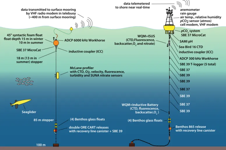
data aNd MethOdS The two moorings, one surface and one subsurface (Figure 1, star), and the glider line (Figure 1, black line), maintained by the University of Washington, are collectively referred to as the Northwest Enhanced Moored Observatory (NEMO); they are part of the Northwest Association of Networked Ocean Observing Systems (NANOOS).

The surface mooring, in 100 m of water

at 47°57'N, 124°58'W, consists of a

UNIX-based buoy controller in a 2 m

discus buoy (Figure 2, right), a suite of

meteorological sensors, a down-looking

300 kHz acoustic Doppler current

profiler (ADCP) to measure full-water-

column currents, and instrumentation

attached at discrete depths along the

main mooring cable to collect a variety of

physical, biological, and chemical mea-

surements. Most relevant to the current

work are the ADCPs, which sample every

five minutes, and Sea-Bird temperature

loggers and MicroCAT conductivity-

temperature-depth (CTD) sensors at 1,

Oceanography | June 2012 71

5, 10, 15, 20, 25, 40, 50, and 60 m depth, which sample every minute. Data are telemetered up the main mooring wire inductively, buffered, archived aboard the buoy controller, and sent back to shore in real time via a Freewave VHF modem.

The shoreside modem is mounted atop a communications tower at the US Coast Guard station 13 nautical miles to the east in La Push, WA, and data are transferred back to the University of Washington from there via Internet.

A McLane moored profiler (MP) on a subsurface mooring 500 m to the north of the surface mooring complements the discrete-depth data from the surface mooring, at the expense of time resolu- tion (Figure 2, left). The MP crawls up

and down the subsurface mooring wire at 25 cm s

between 18 and 92 m depth, completing a profile pair every two hours. Instrumentation includes a Sea-Bird MP52 CTD with a dissolved oxygen sensor, a Falmouth Scientific acoustic current meter, Seapoint fluorometer and turbidity sensors, and a Satlantic Submersible Ultraviolet Nitrate Analyzer (SUNA). The NANOOS MP is the first to carry a nitrate sensor. Data from the subsurface mooring are also telemetered back to shore in real time, via inductive modem to a controller on the subsurface float, to the surface moor- ing via a small “telebuoy” on an L-tether, and back to the Coast Guard station.

In order to provide spatial context

for the mooring observations, we use results from a realistic ocean circulation hindcast model of the region. The 2006 model simulation, described in detail in Sutherland et al. (2011), has been exten- sively validated against data on the shelf;

however, these comparisons mainly focused on subtidal currents and stratifi- cation. The model is forced with realistic wind stress, atmospheric heat flux, rivers, barotropic tides, and subtidal ocean con- ditions on the open boundaries. Notably, it lacks forcing from any open-ocean internal wave field, so the internal tide it develops is due solely to local baro- tropic tide interaction with topography.

The results of this study, given below, demonstrate that the model significantly

inductive coupler (ICC) inductive coupler (ICC)

anemometer rain gauge

air temp., relative humidity p CO2 sensor (atmos) cell modem, VHF modem

85 m stopper 18 m (13 m in

summer) stopper

(4) Benthos glass floats (4) Benthos glass floats

double ORE CART releases with recovery line canister + SBE 39 ADCP 6000 kHz Workhorse

SBE 37 MicroCat

100 m

data transmitted to surface mooring by VHF radio modem in telebuoy (~400 m from surface mooring)

ADCP 300 kHz Workhorse data telemetered

to shore near real-time

SBE 37 MicroCat SAMI pH

SBE 37

SBE 37 SBE 39

SBE 39 T-logger (5 total)

Benthos 865 release with recovery line canister

pCO

system WQM+ISUS

(CTD,Fluorescence, backscatter,O

and nitrate)

SBE 39

SBE 39

SBE 39 Seaglider

WQM+Inductive Battery (CTD, fluorescence, backscatter,O

) McLane profiler

with CTD, O2, velocity, fluorescence, turbidity and SUNA nitrate sensors 45" syntactic foam float

float depth 15 m in winter 10 m in summer

SBE 37 Sea-Bird 16 CTD

figure 2. Schematic of the NeMO system showing the surface mooring (right), the subsurface profiling mooring (left), and the glider.

underestimates the observed energy flux of the internal tide at the mooring, sug- gesting that the neglected internal wave boundary forcing may be important.

The observational systems developed over the past few years will soon be deployed year-round and will be serviced twice yearly as part of the NANOOS pro- gram. This paper describes observations from the first two summertime deploy- ments of the system, in 2010 (surface mooring only) and 2011 (both systems), with a focus on the 2011 measure- ments. The glider data are only used here to provide full-depth stratification information for the flux energy calcula- tions, with the spatial transects deferred for another paper.

OBSerVatIONS

Oceanographic Context

The observed low-frequency currents and stratification are typical of the Washington continental shelf in sum- mer, as described in Hickey (1978) and Hickey and Banas (2003). Winds are predominantly from the northwest (Figure 3a, blue) with periodic south- erly winds typically associated with stormy weather (red periods). Currents (Figure 3b) are generally toward the southeast (135° true), as shown by the time-mean vector plotted in black in Figure 1. One to two days following each of the southerly wind events, currents slacken substantially and even reverse at some depths. The depth average cur- rent (Figure 3c, green) tends to zero during the most substantial of the wind reversals, but it never quite changes sign.

The speed of the low-frequency current varies from ≈ 0 to as great as 0.4 m s

, the same as the group speed of the fastest internal waves in this water depth and

stratification. It is therefore expected that wave propagation should be affected pro- foundly as changing currents advect and refract waves.

Figure 4 examines in more detail the 46-day period after August 8 when the subsurface mooring was profil- ing. Current reversals associated with changes in wind direction are again seen in the velocity plot (Figure 4b). However, at this magnification, the combined semidiurnal barotropic and baroclinic tides appear as regular vertical stria- tions during a 12.4-hour period. The baroclinic tide can be seen as depth- dependent fluctuations in these, and also in the contours of temperature, salinity, and the other scalar fields (Figure 4c–h).

Isopycnals (black) demonstrate the verti- cal motions of the internal tide, which are about 20 m peak-to-peak during the strongest periods.

Temperature, salinity, and stratifica- tion generally respond in the expected way to the low-frequency wind shifts, with the upwelling following each wind burst by one to two days, tending to elevate isopycnals and the other sca- lar fields (e.g., isopycnals rising from August 18–22, then dropping following the downwelling event). The rain gauge on the surface buoy detected 4 cm of rain (not shown) during the August 22 south wind event, which likely also affected shallow stratification.

The semidiurnal fluctuations in velocity and the vertical isopycnal dis- placement tend to weaken during the periods when the current has weakened (e.g., August 23 and September 19), suggesting a connection between the internal waves and the mesoscale flows that will be examined in more detail in later sections. A natural quantity to

examine is the stratification or buoyancy frequency, N, because it has a direct effect on the vertical scales as well as the generation and propagation speeds of the waves. N (Figure 4e) is clearly modulated at these timescales, though not always in a straightforward way. For example, N increases at the surface dur- ing the first two downwelling events, as might be expected, but decreases substantially at depth during the last event, which persists to the end of the record. The complexity is likely at least partly due to three-dimensional effects such as gradients in the along-current/

along-shelf direction.

Figure 4f–h presents dissolved oxy- gen, nitrate, and chlorophyll fields.

Because each quantity depends on bio- logical as well as physical processes, they are considerably more complex than the physical quantities. For example, the record begins with high nitrate and low oxygen in the mixed layer, and nearly no observable chlorophyll. A bloom appears on August 13, coincident with the onset of south winds and weakened current, resulting in high chlorophyll.

Reduced nitrate and increased oxygen

follow, consistent with phytoplankton

growth. The internal tide displace-

ments heave the chlorophyll, oxygen,

and nitrate fields up and down as the

bloom develops. As upwelling resumes,

isopycnals are brought upward, but

nitrate suddenly increases in the upper

30 m on August 22, implying a lateral

transport. Future work will examine the

relative roles of the low-frequency cur-

rents and the internal waves in modulat-

ing these fields.

Oceanography | June 2012 73

7HPSHUDWXUH^R&

9HORFLW\PV^ï

ï

PVï

D:LQGVSHHG 6RXWKZLQGVGRZQZHOOLQJ 1RUWKZHVWZLQGVXSZHOOLQJ

'HSWKP

ï ï

PVï 6HPLGLXUQDO

N-Pï

$3(

PHWHUV

H'RZQZDUGZDYHGLVSODFHPHQW

'DWH 6DPSOHSHULRG

6DPSOHSHULRG

6DPSOHSHULRG

6DPSOHSHULRG

7HPSHUDWXUH

$PSOLWXGHP

3URSDJDWLQJ7RZDUG^RWUXH

9HORFLW\

7HPSHUDWXUH

$PSOLWXGHP

3URSDJDWLQJ7RZDUG^RWUXH

9HORFLW\

7HPSHUDWXUH

$PSOLWXGHP

3URSDJDWLQJ7RZDUG^RWUXH

9HORFLW\

7HPSHUDWXUH

$PSOLWXGHP

3URSDJDWLQJ7RZDUG^RWUXH

9HORFLW\

GHSWKP

GHSWKP GHSWKP

GHSWKP

GHSWKP

GHSWKP

F'HSWKïDYHUDJHGFXUUHQW /RZïIUHTXHQF\

E1RUWKHDVWZDUGFXUUHQWDQGLVRWKHUPV

VSULQJWLGHV

figure 3. a 2011 time series from the surface mooring, with outer insets showing zoom-ins of 18-hour periods around the four times marked in (d) to demonstrate the variability in the internal tide. Inner insets are zoomed in further on the period indicated in each outer inset to illustrate the temperature (top) and baroclinic northward velocity (bottom) of the nonlinear internal waves. (a) Wind speed, colored by direction (south = red, northwest = blue).

(b) Velocity toward 315° true (northwest), with blue colors indicating flow to the southeast. The 8°, 9°, and 10°C isotherms are contoured in gray. (c) depth- averaged velocity towards 315° true (northwest) of the low-frequency flow (green) and the semidiurnal tidal band (blue). (d) Mode-1 semidiurnal tide:

horizontal kinetic energy (hke) and available potential energy (ape) are plotted as stacked histograms, with their sum indicating total energy. energy flux

magnitude in kW m

, which is always toward the north-northeast, is plotted in black. The times of the insets are indicated in red in (d,e). Black dashed lines

in (c–e) show full and new moons, which should correspond with spring tides or maximal semidiurnal tidal forcing. (e) amplitude of the nonlinear internal

waves computed by tracking the depth of the isotherm normally at 15 m depth.

Internal Waves Spectrum

A broad range of frequencies is obvi- ous in both Figures 3 and 4. To quantify the level of the fluctuations at each fre- quency and compare it to other envi- ronments, we compute the spectrum of rotary velocity (Mooers, 1970; Gonella,

1972) using the sine multitaper method of Riedel and Sidorenko (1995). To focus on baroclinic motions, baroclinic velocity u

is first computed by remov- ing the depth mean at each time. By computing the Fourier transform of the time series of u

+ iv

, a frequency spectrum is obtained wherein clockwise

and counterclockwise motions appear at negative and positive frequencies, respectively, which are plotted as blue and green in Figure 5 for 2010 (top) and 2011 (bottom). As expected for internal waves in the Northern Hemisphere, motions are strongly clockwise polar- ized at frequencies near f, becoming unpolarized by about 10 cycles per day.

No prominent near-inertial peak is seen at f, unlike the usual situation in the open ocean. This observation is not surprising given the generally light to moderate winds, because storms are the most efficient generators of near-inertial waves (D’Asaro, 1985). One would expect much stronger near-inertial signals in winter. Instead, semidiurnal and four- times-daily peaks are seen during these summertime records, which are the semidiurnal tide and its “overtide” or first harmonic.

The level of the “continuum” spec- trum between f and N gives the strength of the internal wave field, which is thought to be set by nonlinear inter- actions among the internal waves. In the open ocean, the “GM76” model (Garrett and Munk, 1975, as modified in Cairns and Williams, 1976) provides a framework for comparing continuum levels in different environments. GM76 is over-plotted in gray in Figure 5. For continental shelves, the L02 spectrum (red; Levine, 2002) is more appropri- ate, because it accounts for the effects of the upper and lower boundaries on the waves, but the two spectral forms are nearly identical for our location.

Above the tidal and twice-tidal peaks, the continuum level of the clockwise motions is very close to the L02 and the GM76 model spectra for both 2010 and 2011. At the highest frequencies,

−0.35 0.35

(c) Temperature 0

50 100

°C

7 11

(d) Salinity 0

50 100

psu

31 34

(e) Buoyancy Frequency

Depth (m)Depth (m)Depth (m)Depth (m)Depth (m)Depth (m)Depth (m)

0 50 100

0 12

(f) Dissolved Oxygen 0

50 100

mg l–1µg l–1

0 8

(g) Nitrate 0 50 100

µmol l–1

0 40

(h) Chlorophyll

08/14 08/21 08/28 09/04 09/11 09/18

0 50 100

0 300 (b) Velocity

0 50 100 0 5 10

m s–1 m s–1cph

(a) Wind Speed South Winds: Downwelling Northwest Winds: Upwelling

figure 4. time series of data from the subsurface mooring, corresponding to the last 46 days

of the period plotted in the previous figure. panels are wind speed colored by (a) direction as

in figure 3, (b) velocity toward 315° true, (c) temperature, (d) salinity, (e) buoyancy frequency,

(f) dissolved oxygen, (g) nitrate, and (h) chlorophyll. Isopycnals whose mean spacing is 10 m

are over-plotted in each panel in black.

Oceanography | June 2012 75

the slope flattens and then drops again, which is the signature of the high- frequency waves so evident in the Figure 3 insets. The rise is well above the noise floor of the instrument, which is below the plotting range at about 7 ^× 10

m

s

cpd

. Prior to discussing the high-frequency nonlinear waves, we will next focus on the internal tide and its strength and variability.

Internal Tides

The internal tide contains much of the variance in the velocity spectrum, and so is given special attention in this sec- tion. Four periods of the baroclinic velocity record are plotted in close-up in the Figure 3 insets. Each is an 18-hour period, during which the dominance of motions at a ≈ 12-hour period can be seen. Isotherms measured from the thermistors on the surface mooring are over-plotted in black. Neither veloc- ity nor temperature is filtered, so that the nonlinear waves can be seen (next section). A clear tendency for oppos- ing flow in the upper and lower half of the water column is seen, indicating the dominance of mode-1 motions.

Focusing on the tidal-period motions reveals a general tendency for isotherms to be deflected downward during north- ward flows. This downward deflection of the isotherms is the signature of a wave traveling to the north, because the downward deflection of isopycnals leads to high/low baroclinic pressure in the upper/lower portion of the water column (Althaus et al., 2003). There is, however, considerable variability in the strength of the semidiurnal motions (with the first period showing significantly stronger velocities than the rest), as well as the depth/time structure, with some periods

showing more vertically standing signals, and others (such as the fourth) showing downward phase propagation, implying upward energy propagation.

Quantitative estimates of the energy and energy flux in the internal tide are made following now-standard methods described in Alford (2003), Nash et al.

(2005), and Alford and Zhao (2007a). A modal decomposition is first performed to determine the velocity and vertical displacement amplitude associated with each of the vertical modes discussed in the introduction, where the mode shapes are computed using the time-mean stratification taken from the glider pro- files near the moorings (acknowledging that temporal changes in stratification can lead to errors, as demonstrated by recent work of authors Zhao and Alford

and colleagues). Baroclinic pressure, p

, is then computed by integrating the ver- tical displacement, η(z), in depth, assum- ing motions are hydrostatic (Althaus et al., 2003). The depth-integrated hori- zontal kinetic energy

HKE =

ρ u

dz, available potential energy APE =

ρN

η

dz, and energy flux F =

u

p

dz,

can then be computed. Though semi- diurnal signals dominate, they are nonetheless still isolated via band- pass filtering, using a fourth-order Butterworth filter with cutoffs of 1.7 and 2.3 cycles per day.

ω/cpd 10

10

10

10

10

10

Φ

/m

s

cpd

Φ

/m

s

cpd

ω / cpd

M2 K1 f

2M2

M2 K1 f

2M2 z = 30 m

Year 2010

z = 30 m Year 2011

CW CCW L02 GM76

CW CCW L02 GM76

10

10

10

10

10

figure 5. rotary frequency spectrum of baroclinic velocity at 30 m, measured at the surface

mooring during 2010 (top) and 2011 (bottom). The blue and green curves correspond to

clockwise and counterclockwise motions, respectively. Vertical dashed lines indicate the near-

inertial and tidal frequencies. The levine (2002) and gM76 model spectra are overlain with

red and gray dashed lines, respectively.

These quantities are plotted for the whole period in Figure 3d. As is usual and evident from the insets, the first ver- tical mode dominates both energy and flux. Mode-1 horizontal kinetic energy (HKE) and available potential energy (APE) are plotted as stacked histograms in red and blue, respectively, with mode-1 energy flux magnitude plotted in black.

(Only flux magnitude is plotted because the vector flux is always directed toward the north-northeast.) Energy and energy flux generally rise and fall together, with the ratio near the mode-1 group velocity of 0.4 m s

, as expected for free waves.

However, late in the record, the ratio changes visibly, possibly suggesting inter- ference from waves traveling in different directions (Alford and Zhao, 2007b).

Presumably, these changes are due to the different stratification (as observed in recent work of authors Zhao and Alford and colleagues) and/or currents.

As discussed in the introduction, one would expect semidiurnal energy and flux to rise and fall with the barotropic tidal velocity ^{C –p}

u

H, Δ

, which is estimated as the depth average of the observed semidiurnally band-passed velocity.

Semidiurnal barotropic ellipses are about 0.2 m s

peak-peak and oriented along shelf (Figure 1, gray ellipse), in good agreement with predictions from the TPXO7.2 tidal inverse (Egbert and Erofeeva, 2002). As opposed to the situ- ation in the open ocean, C –p

u

(Figure 3c)

H, Δ shows only a weak spring/neap cycle.

Maxima generally occur near new and full moons (vertical dashed lines), where the astronomical forcing of the semi- diurnal motions is the greatest, but not always (e.g., August 17), indicating the complexity of even barotropic tides in coastal environments.

The baroclinic energy and flux maxima bear little relation to the baro- tropic forcing, suggesting the presence of remotely incident radiation and/

or modulation of the generation and propagation of the local signals by the low-frequency flows. In support of the latter explanation, there is a tendency for flux to be weakest during the periods of weakest northward flow (e.g., July 16, August 23), but the agreement is far from perfect (e.g., September 6). More defini- tive statements may be possible as the length of the time series grows.

The time-mean semidiurnal energy flux is toward the north-northeast in both years, with magnitudes of 86 and 71 W m

, respectively (Figure 1, red arrows). These values are similar to those seen on other continental shelves (e.g., 130 W m

on the New England shelf; MacKinnon and Gregg, 2003b), but much smaller than typical values seen in the open ocean (500 W m

; Alford, 2003a) or near strong sources (as great as 6 ^× 10

W m

; Alford et al., 2011). As an initial examination of the locally generated internal tide field, con- version (colors) and energy flux (blue arrow) are computed from the numeri- cal model. Because the model has no remotely incident internal tide signals, it is representative of the locally gener- ated internal tides. Though caution must be used in interpreting flux direction in multiple sources owing to the presence of interference patterns, model flux at the mooring location appears to emanate from a region of strong convergence west of Juan de Fuca Canyon. By contrast, the observed fluxes in both years (red arrows) are about twice as large as the model fluxes, and are directed more to the north. The observed fluxes that are

stronger than the modeled ones, their lack of an obvious relationship with the local forcing, and the lack of an obvious conversion region to the south-southeast of the mooring all suggest the fluxes are at least partly of remote origin, pos- sibly from Cape Mendocino (Althaus et al., 2003; Alford, 2010) as observed in Oregon (Martini et al., in press), or even Hawaii (Alford and Zhao, 2007a).

Nonlinear Internal Waves

The 18-hour plots shown in the Figure 3 insets (the four corners) show sig- nificant departures from the smooth sinusoids expected for linear waves in both the velocity and temperature sig- nals. To examine these waves in more detail, the 3.5-hour period shown near the center of each plot is replotted in close-up. Sharp waves of depression appear in all four examples as bursts of warm water observed at much greater depth than previously, implying down- ward displacements of 23–38 m in only 100 m of water. Individual waves last 5–10 minutes and are, therefore, well resolved in temperature, which is sam- pled every minute. Assuming the waves are propagating at about the mode-1 phase speed for high-frequency waves of 0.5 m s

, they have horizontal wave- lengths of about 150–300 m.

At times, waves occur singly (sample period #4), or in dramatic sets of many waves as in sample period #2. The decrease in amplitude and spacing of the waves following the first is known as “rank ordering,” and follows from the theory for nonlinear internal waves (see Ostrovsky and Stepanyants, 1989).

Because larger waves travel faster than

smaller waves, they arrive first. The spac-

ing between successive waves decreases

Oceanography | June 2012 77

as the waves get smaller and the speed difference lessens. These characteris- tics are seen in many, but not all, of the waves observed in our data.

The waves show a clear signature in velocity (Figure 3 insets, lower panels), though they are only marginally resolved as velocity is sampled at only five-minute intervals. The baroclinic velocity signa- ture of the waves is mode-1, with each downward displacement accompanied by northward/southward flow in the upper/lower layers. Though only north- ward velocity is plotted in Figure 3, the measured baroclinic velocity vector in the upper 30 m is used to determine propagation direction (indicated for the four examples in the inset), following Ramp et al. (2004). Direction of these and nearly all waves clusters toward the north-northeast, similar to the direc- tion of semidiurnal flux (Figure 1). The NLIW generation mechanism is as yet unknown, but transformations of shoal- ing internal tides into internal bores as they transit the shelf break and/or lee-waves generated by barotropic tides flowing past the shelf break are the most likely candidates. The along-shelf ori- entation of the barotropic tidal ellipses and the propagation of the NLIWs in the same direction as the internal tide are suggestive of the former mechanism, but more work is required to be sure.

The amplitude of the nonlinear waves is computed by tracking the depth of each isotherm relative to a two-day mean, which is intended to represent the slowly varying background state with- out the displacements of internal waves.

The four waves shown in the Figure 3 inset plots range from 23–38 m, in the range of sizes seen on other shelves and continental slopes (Table 1). Expressed

as a fraction of the water depth, the larg- est waves observed on the Washington continental shelf appear to be among the largest anywhere, exceeding even the amplitude-to-depth ratios seen on the South China Sea continental slope.

Though the waves plotted in the Figure 3 insets are among the largest in the record, the full time series of NLIW amplitude (Figure 3e) shows that waves of 20–25 m are common. The magni- tude and frequency of the NLIWs show modulation on a variety of timescales, but appears to bear little relationship with either the barotropic forcing (spring tide times given with dashed lines) or the energy or energy flux of the semidiurnal internal tide (Figure 3d). Waves are at times clearly related to a sharpened front of the downward displacements of the internal tide, as in sample period #1, leading to a sharp decrease/increase in the velocity of the upper/lower lay- ers. However, some waves appear when the internal tide is quite weak, as in sample period #2.

SuMMary aNd dISCuSSION This paper is the first documentation of internal waves on the Washington continental shelf. The internal wave con- tinuum is close to the model spectrum of L02 for continental shelves (Figure 5).

Protruding prominently above this con- tinuum is an active but variable internal tide field (Figure 3, outer insets), and an energetic field of nonlinear waves (Figure 3, inner insets).

The internal tide vertically heaves scalar fields (Figure 4), and propagates toward the north-northeast (Figure 1, red arrows). It appears to be at least partly of remote origin because the observed energy flux is substantially

stronger than in a regional model that includes locally generated tides only. The internal tide is quite variable (Figure 3), displaying neither a clear spring/neap cycle nor an obvious correlation with the local barotropic currents. This observa- tion is some indication that internal tide strength is related to current strength, but more data are required to be sure.

A very energetic NLIW field domi- nates the high-frequency end of the spectrum. NLIWs on the Washington shelf are among the strongest seen on continental shelves (Table 1). They are clearly related to the internal tide, given that they often occur each 12.4 hours.

Like internal tides, NLIWs are directed toward the north-northeast, suggesting that the internal tide possibly gener- ates them via a steepening or related mechanism as described in Colosi et al.

(2001) and Lien et al. (2005). On the other hand, their strength and number appear uncorrelated with either the baro- tropic tidal currents or the energy or flux of the internal tide.

More work is required to determine the origin and generation mechanism of NLIWs. However, their large size makes them potentially important in mixing nutrients upward into the euphotic zone and/or transporting nutrients and larvae laterally on the shelf. Spatial surveys, ideally with microstructure, will be help- ful in determining the generation loca- tion, propagation pathways, and scalar transport of the waves.

aCkNOWledgMeNtS

This work was supported in part by the

National Oceanic and Atmospheric

Administration (NOAA) under IOOS-

NANOOS grant NA11NOS0120036

and the National Science Foundation

under grants OCE0968131 (MA) and OCE 0849622 (PM). The consider- able hardware and instrumentation comprising the surface and subsurface moorings was purchased on a gener- ous grant from the M.J. Murdock Charitable Trust. Discussions with Barbara Hickey and Neil Banas on the Washington coastal environment and ecosystem were extremely helpful. We are grateful to the captain and crew of R/V Thomas G. Thompson for their skill and good attitude in deploying and servicing the moorings. Design and con- struction of the NEMO system would not have been possible without the hard work and engineering expertise of Eric Boget, Mike Carpenter, Mike Kenney, Trina Litchendorf, Keith Magness, Tim McGinnis, Nick Michel-Hart, Zoë Parsons, Chris Siani, and Tim Wen. We are also indebted to Craig Lee and his group for their assistance in piloting the glider. We are grateful to the Coast Guard station in La Push, Washington, for their hospitality and willingness to host our shore data station and to the Quileute Tribe for their hospitality and access. Finally, we would like to thank the Olympic Coast National Marine Sanctuary for their assistance and coop- eration in glider and buoy logistics.

refereNCeS

Alford, M.H. 2003. Redistribution of energy avail- able for ocean mixing by long-range propaga- tion of internal waves. Nature 423:159–163, http://dx.doi.org/10.1038/nature01628.

Alford, M.H. 2010. Sustained, full-water-column observations of internal waves and mixing near Mendocino Escarpment. Journal of Physical Oceanography 40(12):2,643–2,660, http://

dx.doi.org/10.1175/2010JPO4502.1.

Alford, M.H., M.C. Gregg, and M.A. Merrifield.

2006. Structure, propagation and mix- ing of energetic baroclinic tides in Mamala

Bay, Oahu, Hawaii. Journal of Physical Oceanography 36(6):997–1,018, http://

dx.doi.org/10.1175/JPO2877.1.

Alford, M.H., R. Lien, H. Simmons, J.M. Klymak, Y. Yang, D. Tang, and M. Chang. 2010. Speed and evolution of nonlinear internal waves tran- siting the South China Sea. Journal of Physical Oceanography 40(6):1,338–1,355, http://

dx.doi.org/10.1175/2010JPO4388.1.

Alford, M.H., J.A. MacKinnon, J.D. Nash, H.L. Simmons, A. Pickering, J.M. Klymak, R. Pinkel, O. Sun, L. Rainville, R. Musgrave, and others. 2011. Energy flux and dissipation in Luzon Strait: Two tales of two ridges. Journal of Physical Oceanography 41(11):2,211–2,222, http://dx.doi.org/10.1175/JPO-D-11-073.1.

Alford, M.H., and Z. Zhao. 2007a. Global patterns of low-mode internal-wave propagation. Part I:

Energy and energy flux. Journal of Physical Oceanography 37(7):1,829–1,848, http://

dx.doi.org/10.1175/JPO3085.1.

Alford, M.H., and Z. Zhao. 2007b. Global pat- terns of low-mode internal-wave propagation.

Part II: Group velocity. Journal of Physical Oceanography 37(7):1,849–1,858, http://

dx.doi.org/10.1175/JPO3086.1.

Althaus, A., E. Kunze, and T. Sanford. 2003.

Internal tide radiation from Mendocino Escarpment. Journal of Physical Oceanography 33(7):1,510–1,527, http://

dx.doi.org/10.1175/1520-0485(2003)033

<1510:ITRFME>2.0.CO;2.

Apel, J., L. Ostrovsky, Y. Stepanyants, and J. Lynch. 2006. Internal solitons in the ocean.

Woods Hole Oceanographic Institution Technical Report, WHOI-2006-04. Available online at: http://www.dtic.mil/cgi-bin/

GetTRDoc?AD=ADA450369 (accessed May 15, 2012).

Apel, J.R., J.R. Holbrook, A.K. Liu, and J.J. Tsai. 1985. The Sulu Sea internal soli- ton experiment. Journal of Physical Oceanography 15:1,625–1,651, http://

dx.doi.org/10.1175/1520-0485(1985)015

<1625:TSSISE>2.0.CO;2.

Avicola, G.S., J.N. Moum, A. Perlin, and M.D. Levine. 2007. Enhanced turbulence due to the superposition of internal grav- ity waves and a coastal upwelling jet. Journal of Geophysical Research 112, C06024, http://

dx.doi.org/10.1029/2006JC003831.

Bogucki, D., T. Dickey, and L. Redekopp. 1997.

Sediment resuspension and mixing by reso- nantly generated internal solitary waves. Journal of Physical Oceanography 27(7):1,181–1,196, http://dx.doi.org/10.1175/1520-0485(1997) 027<1181:SRAMBR>2.0.CO;2.

Butman, B., P. Alexander, A. Scotti, R. Beardsley, and S. Anderson. 2006. Large internal waves in Massachusetts Bay transport sediments offshore. Continental Shelf Research 26:2,029–2,049, http://dx.doi.org/

10.1016/j.csr.2006.07.022.

Cairns, J.L., and G.O. Williams. 1976. Internal wave observations from a midwater float, 2. Journal of Geophysical Research 81:1,943–1,950, http://

dx.doi.org/10.1029/JC081i012p01943.

Carter, G.S., and M.C. Gregg. 2002. Intense, variable mixing near the head of Monterey Submarine Canyon. Journal of Physical Oceanography 32:3,145–3,165, http://

dx.doi.org/10.1175/1520-0485(2002)032

<3145:IVMNTH>2.0.CO;2.

Colosi, J.A., R.C. Beardsley, J.F. Lynch,

G. Gawarkiewicz, C.S. Chiu, and A. Scotti. 2001.

Observations of nonlinear internal waves on the outer New England continental shelf during the summer Shelfbreak Primer Study. Journal of Geophysical Research 106(C5):9,587–9,601, http://dx.doi.org/10.1029/2000JC900124.

D’Asaro, E. 1985. The energy flux from the wind to near-inertial motions in the mixed layer.

Journal of Physical Oceanography 15:943–959, http://dx.doi.org/10.1175/1520-0485(1985)015

<1043:TEFFTW>2.0.CO;2.

Egbert, G., and S. Erofeeva. 2002. Efficient inverse modeling of barotropic ocean tides. Journal of Atmospheric and Oceanic Technology 19:183–204, http://dx.doi.org/

10.1175/1520-0426(2002)019<0183:EIMOBO>

2.0.CO;2.

Farmer, D., and L. Armi. 1999. The generation and trapping of solitary waves over topography.

Science 283:188–190, http://dx.doi.org/10.1126/

science.283.5399.188.

Farmer, D., Q. Li, and J.-H. Park. 2009. Internal wave observations in the South China Sea: The role of rotation and nonlinearity. Atmosphere- Ocean 47:267–280, http://dx.doi.org/10.3137/

OC313.2009.

Foreman, M., W. Callendar, A. MacFadyen, B. Hickey, R. Thomson, and E. Di Lorenzo.

2008. Modeling the generation of the Juan de Fuca Eddy. Journal of Geophysical Research 113, C03006, http://dx.doi.org/

10.1029/2006JC004082.

Garrett, C.J.R., and W.H. Munk. 1975. Space-time scales of internal waves: A progress report.

Journal of Geophysical Research 80(3):291–297, http://dx.doi.org/10.1029/JC080i003p00291.

Gonella, J. 1972. A rotary-component method for analysing meteorological and oceano- graphic vector time series. Deep-Sea Research 19:833–846, http://dx.doi.org/

10.1016/0011-7471(72)90002-2.

Hickey, B.M. 1978. The California Current System: Hypotheses and facts. Progress in Oceanography 8:191–279, http://dx.doi.org/

10.1016/0079-6611(79)90002-8.

Hickey, B.M., and N.S. Banas. 2003. Oceanography of the US Pacific Northwest coastal ocean and estuaries with application to coastal ecol- ogy. Estuaries 26(4B):1,010–1,031, http://

dx.doi.org/10.1007/BF02803360.

Oceanography | June 2012 79 Hickey, B.M., and N.S. Banas. 2008. Why is the

northern California Current so productive?

Oceanography 21(4):90–107, http://dx.doi.org/

10.5670/oceanog.2008.07.

Horner, R., D. Garrison, and F. Plumley. 1997.

Harmful algal blooms and red tide prob- lems on the US west coast. Limnology and Oceanography 42(5):1,076–1,088, http://

dx.doi.org/10.4319/lo.1997.42.5_part_2.1076.

Jackson, C.R., J.C.B. da Silva, and G. Jeans.

2012. The generation of nonlinear internal waves. Oceanography 25(2):108–123, http://

dx.doi.org/10.5670/oceanog.2012.46.

Kelly, S., and J.D. Nash. 2010. Internal-tide genera- tion and destruction by shoaling internal tides.

Geophysical Research Letters 37, L23611, http://

dx.doi.org/10.1029/2010GL045598.

Klymak, J.M., and J.N. Moum. 2003. Internal soli- tary waves of elevation advancing on a shoaling shelf. Geophysical Research Letters 30(20), 2045, http://dx.doi.org/10.1029/2003GL017706.

Lamb, K. 2002. A numerical investigation of solitary internal waves with trapped cores formed via shoaling. Journal of Fluid Mechanics 451:109–144, http://dx.doi.org/

10.1017/S002211200100636X.

Levine, M. 2002. A modification of the Garrett- Munk internal wave spectrum. Journal of Physical Oceanography 32:3,166–3,181, http://dx.doi.org/10.1175/1520-0485(2002) 032<3166:AMOTGM>2.0.CO;2.

Lien, R., E.A. D’Asaro, F. Henyey, M. Huei Chang, T.Y. Tang, and Y.-J. Yang. 2012.

Trapped core formation within a shoal- ing nonlinear internal wave. Journal of Physical Oceanography 42(4):511–525, http://

dx.doi.org/10.1175/2011JPO4578.1.

Lien, R.-C., T.Y. Tang, M.H. Chang, and E.A. D’Asaro. 2005. Energy of nonlinear inter- nal waves in the South China Sea. Geophysical Research Letters 32, L05615, http://dx.doi.org/

10.1029/2004GL022012.

Lighthill, J. 1978. Waves in Fluids. Cambridge University Press, New York, 496 pp.

Lucas, A., P. Franks, and C. Dupont. 2011.

Horizontal internal-tide fluxes support elevated phytoplankton productivity over the inner continental shelf. Limnology & Oceanography:

Fluids & Environments 1:56–74, http://lofe.

dukejournals.org/content/1/56.full.pdf.

MacFadyen, A., and B.M. Hickey. 2010.

Generation and evolution of a topographi- cally linked, mesoscale eddy under steady and variable wind-forcing. Continental Shelf Research 30(13):1,387–1,402, http://dx.doi.org/

10.1016/j.csr.2010.04.001.

MacKinnon, J.A., and M.C. Gregg. 2003a. Mixing on the late-summer New England Shelf:

Solibores, shear, and stratification. Journal of Physical Oceanography 33:1,476–1,492, http://dx.doi.org/10.1175/1520-0485(2003) 033<1476:MOTLNE>2.0.CO;2.

MacKinnon, J.A., and M.C. Gregg. 2003b.

Shear and baroclinic energy flux on the summer New England Shelf. Journal of Physical Oceanography 33:1,462–1,475, http://dx.doi.org/10.1175/1520-0485(2003) 033<1462:SABEFO>2.0.CO;2.

Martini, K.I., M.H. Alford, S. Kelly, and J.D. Nash.

2011. Observations of internal tides on the Oregon continental slope. Journal of Physical Oceanography 41(9):1,772–1,794, http://

dx.doi.org/10.1175/2011JPO4581.1.

Martini, K.I., M.H. Alford, S. Kelly, and J.D. Nash.

In press. Observations of remotely generated internal tides breaking on the Oregon continen- tal slope. Journal of Physical Oceanography.

Maxworthy, T. 1980. On the formation of nonlinear internal waves from the gravitational collapse of mixed regions in two and three dimensions.

Journal of Fluid Mechanics 96(1):47–64, http://

dx.doi.org/10.1017/S0022112080002017.

Mooers, C.N.K. 1970. The Interaction of an Internal Tide with the Frontal Zone in a Coastal Upwelling Region. PhD thesis, Oregon State University.

Nagovitsyn, A., E. Pelinovsky, and Y. Stepanyants.

1991. Observation and analysis of soli- tary internal waves in the coastal zone of the Sea of Okhotsk. Journal of Physical Oceanography 2(1):65–70, http://dx.doi.org/

10.1007/BF02197419.

Nash, J.D., M.H. Alford, and E. Kunze. 2005.

Estimating internal-wave energy fluxes in the ocean. Journal of Atmospheric and Oceanic Technology 22(10):1,551–1,570, http://

dx.doi.org/10.1175/JTECH1784.1.

Nash, J.D., and J. Moum. 2005. River plumes as a source of large-amplitude internal waves in the coastal ocean. Nature 437:400–403, http://

dx.doi.org/10.1038/nature03936.

Nash, J.D., E.L. Shroyer, S.M. Kelly, M.E. Inall, T.F. Duda, M.D. Levine, N.L. Jones, and R.C. Musgrave. 2012. Are any coastal internal tides predictable? Oceanography 25(2):80–95, http://dx.doi.org/10.5670/oceanog.2012.44.

Ostrovsky, L.A., and Y. Stepanyants. 1989. Do internal solitons exist in the ocean? Journal of Geophysical Research 27:2,906–2,926, http://

dx.doi.org/10.1029/RG027i003p00293.

Pineda, J. 1999. Circulation and larval distribution in internal tidal bore warm fronts. Limnology and Oceanography 44(6):1,400–1,414, http://

dx.doi.org/10.4319/lo.1999.44.6.1400.

Pingree, R.D., and A.L. New. 1989. Downward propagation of internal tide energy into the Bay of Biscay. Deep-Sea Research Part I 36(5):735–758, http://dx.doi.org/

10.1016/0198-0149(89)90148-9.

Rainville, L., and R. Pinkel. 2006.

Propagation of low-mode internal waves through the ocean. Journal of Physical Oceanography 36:1,220–1,236, http://

dx.doi.org/10.1175/JPO2889.1.

Ramp, S.R., D. Tang, T.F. Duda, J.F. Lynch, A.K. Liu, C.S. Chiu, F. Bahr, Y.R. Kim, and Y.J. Yang. 2004. Internal solitons in the north- eastern South China Sea. Part I: Sources and deep water propagation. IEEE Journal of Oceanic Engineering 29(4):1,157–1,181, http://

dx.doi.org/10.1109/JOE.2004.840839.

Riedel, K.S., and A. Sidorenko. 1995. Minimum bias multiple taper spectral estimation. IEEE Transactions on Signal Processing 43(1):188–195, http://dx.doi.org/10.1109/78.365298.

Sabine, C.L., R.A. Feely, N. Gruber, R.M. Key, K. Lee, J.L. Bullister, R. Wanninkhof, C.S. Wong, D.W.R. Wallace, B. Tilbrook, and others. 2004.

The oceanic sink for anthropogenic CO

. Science 305:367–371, http://dx.doi.org/10.1126/

science.1097403.

Sandstrom, H., and J.A. Elliott. 1984. Internal tide and solitons on the Scotian shelf: A nutri- ent pump at work. Journal of Geophysical Research 89(C4):6,415–6,426, http://dx.doi.org/

10.1029/JC089iC04p06415.

Sandstrom, H., and N.S. Oakey. 1995. Dissipation in internal tides and solitary waves. Journal of Physical Oceanography 25:604–614, http://

dx.doi.org/10.1175/1520-0485(1995)025

<0604:DIITAS>2.0.CO;2.

Scotti, A., and J. Pineda. 2004. Observation of very large and steep internal waves of eleva- tion near the Massachusetts coast. Geophysical Research Letters 31, L22307, http://dx.doi.org/

10.1029/2004GL021052.

Shroyer, E., J. Moum, and J. Nash. 2011.

Nonlinear internal waves over New Jersey’s continental shelf. Journal of Geophysical Research 116, C03022, http://dx.doi.org/

10.1029/2010JC006332.

St. Laurent, L., and C. Garrett. 2002. The role of internal tides in mixing the deep ocean. Journal of Physical Oceanography 32(10):2,882–2,899, http://dx.doi.org/10.1175/1520-0485(2002)032

<2882:TROITI>2.0.CO;2.

St. Laurent, L.C., H.L. Simmons, T.Y. Tang, and Y.H. Wang. 2011. Turbulent properties of internal waves in the South China Sea.

Oceanography 24(4):78–87, http://dx.doi.org/

10.5670/oceanog.2011.96.

Sutherland, D.A., P. MacCready, N.S. Banas, and L.F. Smedstad. 2011. A model study of the Salish Sea estuarine circulation. Journal of Physical Oceanography 41(6):1,125–1,143, http://dx.doi.org/10.1175/2011JPO4540.1.

Whitney, F.A., H.J. Freeland, and M. Robert. 2008.

Persistently declining oxygen levels in the interior waters of the eastern subarctic Pacific.

Progress in Oceanography 7(2):179–199, http://

dx.doi.org/10.1016/j.pocean.2007.08.007.

Zhao, Z., and M.H. Alford. 2009. New altimetric estimates of mode-one M

internal tides in the Central North Pacific Ocean. Journal of Physical Oceanography 39:1,669–1,684, http://

dx.doi.org/10.1175/2009JPO3922.1.