Exact Algorithms for 0-1 Integer Programs with Linear Equality Constraints

全文

(1)Vol.2014-AL-148 No.10 2014/6/13. IPSJ SIG Technical Report. Exact Algorithms for 0-1 Integer Programs with Linear Equality Constraints Kenya Ueno1,a). Abstract: In this paper, we show an O(1.415n )-time exact algorithm for the feasibility problem of 0-1 integer programs whose constraints are only linear equalities. The algorithm is quadratically faster than exhaustive search and also almost quadratically faster than the algorithm for an inequality version of the feasibility problem by Impagliazzo, Lovett, Paturi and Schneider (arXiv:1401.5512), which motivated our work. Rather than improving the time complexity, we advance to a simple direction as inclusion of many NP-hard problems in terms of exact exponential algorithms. We also extend our algorithm to the optimization problem of 0-1 integer programs with linear equality constraints.. 1. Introduction 1.1 The Feasibility Problem The existence of integer solutions for a certain system of equations has been discussed as one of the fundamental problems in the theory of computation. A prominent example is the Hilbert 10th problem on Diophantine equations [14]. In this paper, we study the feasibility problem of 0-1 integer programs whose constraints are only linear equalities as follows: Problem 1.1 (Feasibility of 0-1 Integer Programs with Linear Equalities). Find x ∈ {0, 1}n which satisfies a given set of linear equalities Ax = b. We give an exact exponential algorithm running in O(1.415n )time and thus achieve a quadratic speedup compared to exhaustive search (brute-force search) running in O(2n )-time. Our algorithm can store the data of all the feasible solutions in O(1.415n )space, even if the number of solutions is more than O(1.415n ). The problem can be seen as a database search where the structured set of data is given by B = {b | Ax = b and x ∈ {0, 1}n }. As s similar problem, there is a quantum algorithm known as Grover’s algorithm, which can achieve quadratic speedup for the unstructured database search problem [9]. The Grover’s algorithm gives a correct answer with high probability, but our algorithm do not use randomness and always gives a correct answer. Recently, probabilistic polynomial algorithms solving a system of linear equations has been discussed by Raghavendra [16] and Fliege [5]. If we eliminate the 0-1 constraints, we can give a polynomial time algorithm by the Gaussian elimination. 1.2 The Optimization Problem Then, we extend our algorithm for the following standard optimization problem running in O(1.415n )-time: 1 a). The Hakubi Center for Advanced Research, Kyoto University kenya@i.kyoto-u.ac.jp. c 2014 Information Processing Society of Japan ⃝. Problem 1.2 (Optimization of 0-1 Integer Programs with Linear Equalities). min s.t.. cT x Ax = b, x ∈ {0, 1}n .. We know that there are many sophisticated ideas (e.g., the branch-and-bound method and the cutting-plane method) improving algorithms and implementations for computing 0-1 integer programs [8], [15]. However, there are no improvements of worst-case time complexity for integer programs from the exhaustive search to the best of our knowledge. 1.3 Exact Algorithms for NP-hard Problems: Since there are no polynomial time algorithms for NP-hard problems unless P=NP, many researchers have studied exact exponential time algorithms which are faster than exhaustive search for NP-hard problems [6], [11], [13], [19]. Integer programs include many NP-hard problems as special cases [7]. For instance, the subset sum problem is a special case of Problem 1.1 in which the number of constraints is exactly one. Among several such problems whose exact algorithms have been studied, some problems (e.g., the subset sum problem [17]) have the same time complexity as Problem 1.1, and some other problems (e.g., the exact satisfiability problem [3] and the exact hitting set problem [4]) have algorithms faster than O(1.415n )time. In particular, the exact satisfiability problem, which is also a special case of Problem 1.1, has been intensively studied by several researchers [3], [4]. On the other hand, it seems to be difficult to improve the time complexity of our algorithms due to a similar reason of NPhardness. In other words, if we can improve our algorithms, then we simultaneously improve the time complexity of exact algorithms for many NP-hard problems which can be reduced to Problem 1.1. 1.

(2) Vol.2014-AL-148 No.10 2014/6/13. IPSJ SIG Technical Report. 1.4 Circuit Lower Bounds from Moderately Exponential Algorithms Very recently, Impagliazzo, Lovett, Paturi and Schneider [10] studied the feasibility problem for the inequality version of 0-1 integer programs stated as follows: Problem 1.3 (Feasibility of 0-1 Integer Programs with Linear Inequalities). Find x ∈ {0, 1}n which satisfies a given set of linear inequalities Ax ≥ b. Impagliazzo, Lovett, Paturi and Schneider [10] gave an algorithm solving Problem 1.3 in O(2(1−poly(1/c))n) )-time where cn is the number of constraints. It improves an algorithm for Problem 1.3 by Impagliazzo, Paturi and Schneider [12], which is faster than O(2n )-time only when the number of inequalities is smaller than 0.136n. The work by Impagliazzo, Paturi and Schneider [12] is motivated from the challenge initiated by Williams [18] for proving lower bounds for certain circuit models. In this context, it is important to give only a modest improvement of the exponential factor from the O(2n )-time exhaustive search. 1.5 Our Techniques Our algorithms are built on a simple combination of basic techniques on exact algorithms for NP-hard problems. In particular, we use a classic technique called the 2-table method studied in [17]. This method splits n-variables into the two sets of n/2variables, and lists all possible 2n/2 -assignments for each set. This preprocessing enables us to give algorithms which run faster than O(2n )-time for certain problems. On the other hand, there are some technical problems to apply the method to Problem 1.1. One problem is how we construct the 2-table for algorithms. Another problem is how we give analysis to bound the time complexity The ideas introduced in the two papers [10], [12] allow us to overcome these technical problems. To construct the 2-table for Problem 1.1 and 1.2, we introduce a notion of the vector equality problem, a variation of the vector domination problem studied by Impagliazzo, Paturi and Schneider [12]. To analyze the time complexity, we need to incorporate an idea using the weighted median (or the weighted sorting), which is introduced very recently by Impagliazzo, Lovett, Paturi and Schneider [10]. Furthermore, we complete our analysis of the time complexity by setting a suitable choice of complexity measure, which is a novel point of this paper, for the search space in the 2-table method. Another novel point is an extension of the feasibility problem to the optimization problem by using the 2-table method. This is achieved by post-processing after solving the feasibility problem with extra storage of the objective function. There are no extra blow-up of the exponential time complexity. We hope that our contribution will be useful in practice as well as theoretical analysis of algorithms. 1.6 Organization of This Paper This paper is organized as follows. In Section 3, we introduce a notion of the vector equality problem and show a recursive algorithm solving the problem. Then, we give analysis of its time. c 2014 Information Processing Society of Japan ⃝. complexity. In Section 4, we describe how we solve the feasibility problem and the optimization problem by reducing them to the vector equality problem. In the last section, we conclude this paper and list some open problems.. 2. Notations Throughout the paper, we use the following notations. We denote m × n constant matrices by A, and i, j-th element of a matrix A by Ai, j . We use b and c as constant vectors. cT is the transpose of c. We also use x, u and v as variable vectors. We denote j-th element of a vector x by x j . The same notation applies for other constant and variable vectors. The function poly(n) is some polynomial for n. Following the convention in the theory of exact algorithms, we measure the time complexity by the function of n, which is the number of variables. We assume m ∈ O(poly(n)) since otherwise the input size is super-polynomial to n.. 3. The Vector Equality Problem In this section, we consider the following problem: Definition 3.1 (Vector Equality). Given two sets of mdimensional vectors U and V, the vector equality problem is the problem of finding two vectors u ∈ U and v ∈ V such that u = v. To solve the vector equality problem efficiently, we need to use a notion of the weighted median to bound the time complexity of our algorithms. Definition 3.2 (Weighted Median). The weighted median for a set of weighted numbers is a number such that both the total weight of numbers smaller than the weighted median and the total weight of numbers larger than the weighted median are at most half of the total weight of all the numbers. Then, we consider the following recursive algorithm (Algorithm 1) computing the vector equality problem. Following a linear time algorithm for the unweighted median problem [2], we can give a linear time algorithm for the weighted median problem [1], which is also indicated in [10]. Lemma 3.3 ([1], [10]). The weighted median of N numbers can be computed in O(N)-time. In the next section, we will give algorithms for 0-1 integer programs with linear equality constraints by reducing them to the vector equality problem. Before that, we analyze the time complexity of Algorithm 1 for the vector equality problem in the following lemma. Lemma 3.4. The vector equality problem can be computed in O(mN log N)-time where |U| = |V| = N by starting Algorithm 1 at VectorEquality(U, V, 1, m). Proof. In Algorithm 1, we find the weighted median k of the ith coordinates of U ∪ V where all the elements in U and V have weight |V| and |U|, respectively. Then, we partition U into three sets: U + = {u | ui > k}, U = = {u | ui = k}, U − = {u | ui < k}. 2.

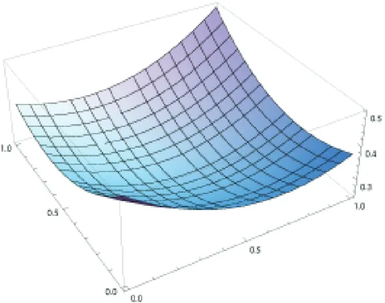
(3) Vol.2014-AL-148 No.10 2014/6/13. IPSJ SIG Technical Report. Algorithm 1 VectorEquality(U, V, i, m) Require: Two sets of m-dimensional vectors and an index i and the dimension m Ensure: A list of two sets of m-dimensional vectors if U = ∅ or V = ∅ then return an empty list else if i > m then return a singleton list of (U, V) else (1) Find the weighted median k of the i-th coordinates of U ∪ V with weight |V| and |U| for each element in U and V, respectively. (2) Partition U into three sets: (a) U + = {u | ui > k}, (b) U = = {u | ui = k}, (c) U − = {u | ui < k}. (3) Partition V into three sets: (a) V + = {u | vi > k}, (b) V = = {u | vi = k}, (c) V − = {u | vi < k}. (4) Solve the following three subproblems: (a) L1 = VectorEquality(U + , V + , i, m) (b) L2 = VectorEquality(U = , V = , i + 1, m) (c) L3 = VectorEquality(U − , V − , i, m) return the concatenation of the three lists L1, L2, and L3 end if. √ α + β ≥ 2 αβ for any α, β ≥ 0, we have. We also partition V into three sets:. |U + | |U| |U − | |U| |U = | |U|. V + = {u | vi > k}, V = = {u | vi = k}, V − = {u | vi < k}. Two vectors u ∈ U and v ∈ V can be equal in one of the following three cases: (1) u ∈ U + and v ∈ V + , (2) u ∈ U = and v ∈ V = , (3) u ∈ U − and v ∈ V − .. =. −. +. =. −. |V| · (|U | + |U | + |U |) + |U| · (|V | + |V | + |V |) =|V| · |U| + |U| · |V|. Dividing it by |U| · |V|, we have |U + | + |U = | + |U − | |V + | + |V = | + |V − | + = 2. |U| |V| For some constants s and t such that 0 ≤ s ≤ 1 and 0 ≤ t ≤ 1, we have |U + | |V + | + = 1 − s, |U| |V| |U − | |V − | + = 1 − t, |U| |V| |U = | |V = | + = s+t |U| |V| because we partitioned U and V at the weighted median. Since. c 2014 Information Processing Society of Japan ⃝. Collecting these inequalities, we have |U + | · |V + | · 2m + |U − | · |V − | · 2m + |U = | · |V = | · 2m−1. We solve smaller subproblems of the vector equality problem for the three cases as in Figure 1. In particular, we decrease the dimension m to m − 1 in the case of (2). The rule of the partition immediately gives the following equation: +. |V + | 1 ≤ · (1 − s)2 , |V| 4 |V − | 1 · ≤ · (1 − t)2 , |V| 4 |V = | 1 · ≤ · (s + t)2 . |V| 4 ·. 1 ≤ · {(1 − s)2 · 2m + (1 − t)2 · 2m + (s + t)2 · 2m−1 } · |U| · |V| 4 1 1 = · {(1 − s)2 + (1 − t)2 + · (s + t)2 } · |U| · |V| · 2m . 4 2 It means that the search space |U| · |V| · 2m decreases by the factor of 1 1 · {(1 − s)2 + (1 − t)2 + (s + t)2 } 4 2 = 0.5 − 0.5s − 0.5t + 0.375s2 + 0.375t2 + 0.25st. f (s, t) =. at each recursion. We can conclude f (s, t) ≤ 12 in the domain of 0 ≤ s ≤ 1 and 0 ≤ t ≤ 1 as in Figure 2. Strictly speaking, we can formally analyze by taking the partial derivatives, ∂ f (s, t) = −0.5 + 0.75s + 0.25t, ∂s ∂ f (s, t) = −0.5 + 0.25s + 0.75t. ∂t (s,t) If ∂ f∂s > 0 (equivalently, t > 2 − 3s), then the function f (s, t) (s,t) is monotonically increasing in the direction of s. If ∂ f∂s < 0 (equivalently, t < 2 − 3s), then the function f (s, t) is monotonically decreasing in the direction of s. The same thing applies for t instead of s.. 3.

(4) Vol.2014-AL-148 No.10 2014/6/13. IPSJ SIG Technical Report. V+. V=. V−. U+. U=. U−. Fig. 1. Fig. 2. c 2014 Information Processing Society of Japan ⃝. Partition of the Two Sets of Vectors U and V. f (s, t) = 0.5 − 0.5s − 0.5t + 0.375s2 + 0.375t2 + 0.25st. 4.

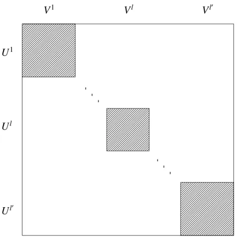
(5) Vol.2014-AL-148 No.10 2014/6/13. IPSJ SIG Technical Report. Therefore, we can verify that it is maximized at two edges (s, t) = (0, 0), (1, 1) as f (s, t) = 0.5 and minimized at the middle point (s, t) = (0.5, 0.5) as f (s, t) = 0.25. Moreover, maximal points except the two edges are only two points (s, t) = (0, 1), (1, 0) as f (s, t) = 0.375. The recursions occur at most log2 (|U| · |V| · 2m ) ∈ O(m log N) depth. At each depth d of the recursion, we need to solve at most 3d (< N) subproblems of the vector equality problem, but the total number of elements is at most 2N. Therefore, we can solve the weighted median in linear time O(|U| + |V|) = O(N) as a whole at each depth of the recursion. As a consequence, we conclude that the total time complexity of Algorithm 1 is O(mN log N). □ Instead of the algorithm for the weighted median, we can use a sorting algorithm running in O(N log N)-time. More precisely, we can find the weighted median by looking at the middle element which divide the total weights to less than or equal to its half after sorting the weighted elements. In this case, the time complexity of the algorithm becomes worse as O(mN log2 N), but the time bound will be steady for our main algorithms for 0-1 integer programs with linear equality constraints to be shown in the next section.. 4. Exact Algorithms for 0-1 Integer Programs In this section, we give exact algorithm for solving the feasibility and optimization problem of 0-1 integer programs with linear equality constraints. Each algorithm is given by reducing it to the vector equality problem described in the previous section. 4.1 The Feasibility Problem First, we give the algorithm for 0-1 integer programs with linear equality constraints by showing the following theorem. Theorem 4.1. The feasibility problem of 0-1 integer programs with linear equalities (Problem 1.1) can be computed in O(m · 2n/2 poly(n))-time. Proof. Unlike the inequality problem, the equality problem has at most n independent equations. Otherwise, a set of solutions x ∈ {0, 1}n must be empty. We assume the number of variables n is even without loss of generality. We solve the feasibility problem of Ax = b by reducing it to the vector equality problem. First, we partition the set of variables X = {x1 , · · · , xn } into two disjoint subsets X1 and X2 . Let α(x j ) and β(x j ) be assignments of x j ∈ X1 and x j ∈ X2 , respectively. Then, we define vectors u and v by ∑ ui = Ai j · α(x j ), x j ∈X1. vi = bi −. ∑. V in O(mN log N)-time by using Algorithm 1. Consequently, we have an algorithm for the feasibility problem of Ax = b running in O(m · 2n/2 poly(n))-time. □ Since the polynomial function is bounded as poly(n) ∈ O(ϵ n ) for any constant ϵ > 1 and m ∈ O(poly(n)) is assumed, the following upper bound is obtained. Corollary 4.2. The feasibility problem of 0-1 integer programs with linear equalities (Problem 1.1) can be computed in O(1.415n )-time. Our algorithm can enumerate all the possible solutions. If the number of solutions is bounded by O(n1.415 ), then the time complexity is also O(n1.415 ). If the number of solutions is ω(n1.415 ), then the time complexity depends on the number of possible solutions. It may sound strange that we can store the data of all possible solutions within O(n1.415 )-space, even if the number of all possible solutions is ω(n1.415 ). This is just because we store the data as a collection of partitioned matrices as in Figure 3. 4.2 The Optimization Problem Taking into account the linearity of the objective function cT x of Problem 1.2, we can extend the algorithm for the feasibility problem to one for the optimization problem. Theorem 4.3. The optimization problem of 0-1 integer programs with linear equalities (Problem 1.2) can be computed in O(m · 2n/2 poly(n))-time. Proof. We essentially follow the algorithm for the feasibility problem and solve the optimization problem by reducing it to the vector equality problem. We partition the set of variables X = {x1 , · · · , xn } into two disjoint subsets X1 and X2 . Let α(x j ) and β(x j ) be assignments of x j ∈ X1 and x j ∈ X2 , respectively. Then, we define vectors u and v by ∑ ui = Ai j · α(x j ), x j ∈X1. vi = bi −. ∑. Ai j · β(x j ).. x j ∈X2. for each assignment of X1 and X2 . Let U and V be two sets of 2n/2 such vectors u and v, respectively. The point which is different from Theorem 4.1 is that we additionally calculate weight ∑ w(u) = c j · α(x j ), x j ∈X1. w(v) =. ∑. c j · β(x j ). x j ∈X2. Ai j · β(x j ).. x j ∈X2. for each assignment of X1 and X2 . Let U and V be two sets of 2n/2 such vectors u and v, respectively. From the construction of U and V, there is a 0,1-vector x ∈ {0, 1}n satisfying Ax = b if and only if there is a pair of two vectors u ∈ U and v ∈ V satisfying ui = vi for all i (1 ≤ i ≤ m). Therefore, we can solve the vector equality problem for U and. c 2014 Information Processing Society of Japan ⃝. for each of u ∈ U and v ∈ V, respectively. Then, we solve the vector equality problem for U and V by Algorithm 1. After Algorithm 1 terminates, we can get a list of submatrices which contains information of all the possible solutions. ′. ′. (U 1 , V 1 ), (U 2 , V 2 ), · · · , (U l , V l ), · · · , (U l , V l ) There are at most N = 2n/2 submatrices. From the construction 5.

(6) Vol.2014-AL-148 No.10 2014/6/13. IPSJ SIG Technical Report. V1. Vl. Vl. ′. U1. Ul. Ul. ′. Fig. 3. A List of Submatrices from Algorithm 1 for the Vector Equality Problem. of Algorithm 1, each row and column of submatrices has no intersection. Let U l × V l (U l ⊆ U and V l ⊆ V) be one of such submatrices. Then we would like to solve the following optimization problem for each l. min s.t.. w(u) + w(v) u ∈ U l and v ∈ V l .. From the linearity of cT , w(u) and w(v) are independent. Therefore , the above minimization problem is solvable separately for u and v. Hence, O(|U l | + |V l |)-time is sufficient to optimize. We solve the same problem for each submatrices and take the minimum of all the problems. The total time complexity is O(m · 2n/2 poly(n)). □ Corollary 4.4. The optimization problem of 0-1 integer programs with linear equalities (Problem 1.2) can be computed in O(1.415n )-time.. 5. Conclusions and Open Problems In this paper, we have studied O(1.415n )-time exact algorithms for 0-1 integer programs with linear equality constraints. We can apply our algorithms to not only the feasibility problem but also the optimization problem. We can also extend our algorithms to integer programs where the variables are constrained by any finite set of values, although we don’t treat them in this paper. There are some open problems. c 2014 Information Processing Society of Japan ⃝. remained as follows. • Shroeppel and Shamir [17] studied the k-table method, which is a generalization of the 2-table method, and showed an O(2n/4 )-space exact algorithm for the subset sum problem by using the 4-table method. However, we don’t know how we utilize the potential of the k-table method for 0-1 integer programs at the moment. Such extensions may lead further improvement of our algorithms and will be interesting research directions. • The algorithm for the inequality version of the feasibility problem of 0-1 integer programs by Impagliazzo, Paturi and Schneider [12] is motivate from the attempts to prove lower bounds for restricted circuit models [18]. We don’t know where there is any restricted circuit models corresponding to the equality version of the feasibility problem. This may be an interesting open question to investigate. • Since our algorithms are very simple, we expect that they will be also useful from the practical point of view. One of important tasks as future works is to give a computational experiment and performance analysis in practice. We hope that our techniques will be useful in both theoretical and practical aspects of algorithms.. Acknowledgment This work is supported by Grant-in-Aid for Young Scientists (B) (JSPS KAKENHI Grant Number 24700010), and Grant-in-Aid. 6.

(7) IPSJ SIG Technical Report. Vol.2014-AL-148 No.10 2014/6/13. for Scientific Research on Innovative Areas (MEXT KAKENHI Grant Number 24106006). References [1]. [2]. [3] [4] [5] [6] [7] [8] [9] [10] [11] [12]. [13] [14] [15] [16] [17] [18] [19]. Bleich, C. and Overton, M.: A linear-time algorithm for the weighted median problem, Technical Report 75, Computer Science Department, Courant Institute of Mathematical Sciences, New York University (1983). Blum, M., Floyd, R. W., Pratt, V., Rivest, R. L. and Tarjan, R. E.: Linear time bounds for median computations, Proceedings of the 40th annual ACM symposium on Theory of computing (STOC 1972), ACM, pp. 119–124 (1972). Byskov, J. M., Madsen, B. A. and Skjernaa, B.: New algorithms for exact satisfiability, Theoretical Computer Science, Vol. 332, No. 1, pp. 515–541 (2005). Drori, L. and Peleg, D.: Faster exact solutions for some NP-hard problems, Theoretical Computer Science, Vol. 287, No. 2, pp. 473–499 (2002). Fliege, J.: A randomized parallel algorithm with run time O(n2 ) for solving an n × n system of linear equations, arXiv preprin arXiv:1209.3995 (2012). Fomin, F. V. and Kratsch, D.: Exact exponential algorithms, Springer (2010). Garey, M. R. and Johnson, D. S.: Computers and intractability; a guide to the theory of NP-completeness, W.H. Freeman (1979). Genova, K. and Guliashki, V.: Linear integer programming methods and approaches – a survey, Journal of Cybernetics and Information Technologies, Vol. 11, No. 1 (2011). Grover, L. K.: A fast quantum mechanical algorithm for database search, Proceedings of the 28th Annual ACM Symposium on Theory of Computing (STOC 1996), ACM, pp. 212–219 (1996). Impagliazzo, R., Lovett, S., Paturi, R. and Schneider, S.: 0-1 Integer Linear Programming with a Linear Number of Constraints, arXiv preprint arXiv:1401.5512 (2014). Impagliazzo, R. and Paturi, R.: On the Complexity of k-SAT, Journal of Computer and System Sciences, Vol. 62, No. 2, pp. 367–375 (2001). Impagliazzo, R., Paturi, R. and Schneider, S.: A satisfiability algorithm for sparse depth two threshold circuits, Proceedings of the 54th Annual Symposium on the Foundations of Computer Science (FOCS 2013), IEEE, pp. 479–488 (2013). Impagliazzo, R., Paturi, R. and Zane, F.: Which Problems Have Strongly Exponential Complexity?, Journal of Computer and System Sciences, Vol. 63, No. 4, pp. 512–530 (2001). Matiyasevich, Y.: Hilbert’s 10th Problem, The MIT Press (1993). Nemhauser, G. L. and Wolsey, L. A.: Integer and Combinatorial Optimization, John Wiley and Sons (1988). Raghavendra, P.: A Randomized Algorithm for Linear Equations over Prime Fields, Manuscript (2012). Schroeppel, R. and Shamir, A.: A T = O(2n/2 ), S = O(2n/4 ) Algorithm for Certain NP-Complete Problems, SIAM journal on Computing, Vol. 10, No. 3, pp. 456–464 (1981). Williams, R.: Improving exhaustive search implies superpolynomial lower bounds, SIAM Journal on Computing, Vol. 42, No. 3, pp. 1218– 1244 (2013). Woeginger, G. J.: Exact algorithms for NP-hard problems: A survey, Combinatorial Optimization – Eureka, You Shrink!, Springer, pp. 185– 207 (2003).. c 2014 Information Processing Society of Japan ⃝. 7.

(8)