複数視点から撮影した海底音響画像を用いた海底物体の三次元構造の再構成
8
0
0
全文
(2) コンピュータビジョンとイメージメディア 134−5 (2002. 9. 12). I. INTRODUCTION For ocean investigation, it has become an important technology to use the underwater acoustic imaging with the side-scan sonar [1-3]. But since typical side-scan sonar is poor for determining accurate bathymetric positions [4], its application was limited in 2-D analysis such as observation, segmentation and classification of seabed [1, 2, 5]. For 3-D analysis, we usually have to deploy multi-beam sonar to obtain the bathymetric measures [6]. This technology, based on beam-forming, often has less spatial resolution capability, map smaller sectors, so it leads to increase the costs of investigation [7, 8]. As we know, getting the information about 3-D structure of the seabed is important for safe navigation, positioning of offshore installations such as oil platforms or oil and gas pipes, recognition of topographical features of the seabed etc., so it becomes necessary to find more efficient method. At present, several approaches are developed. Johnson and Herbert applied shape from shading techniques to reconstruct elevation maps of the seabed from side-scan sonar backscatter images and sparse bathymetric points co-registered within the image [9, 10]. This method depends on a scattering model, so depth information was not necessary. But some of the scattering parameters have to be estimated correctly and some parameters have to be set up empirically. Zerr and Stage developed an algorithm to compute the volume information from the shadow information obtained from a sequence of sonar images [11]. Dura, Lane, and Bell extended this work to automatic 3-D reconstruction of mine geometry [12]. In these approaches, only a few sonar parameters, such as the altitude and range are needed and the computational requirements are lower. But the shadow information couldn’t always be obtained. In this paper we focus on how to reconstruct a 3D structure of the seabed from a spatial series of the 2-D underwater acoustic images. We use a combination of the GPS positioning and the image matching technology to synthesize two or more different underwater acoustic images taken from different viewpoints, and then extract the range data from the spatial series of underwater acoustic images. According to the relation of the spatial position we can estimate 3-D structure with these range data. The rest of the paper is organized as follows. In Section 2 we present our basic idea. We describe the algorithms for tracking the side-scan sonar and. determining the frames of corresponding subimages in Section 3. We detail in Section 4, the method of multi-step gray-level projective matching. Then, in Section 5, we report experimental result. Finally, a discussion and concluding remarks are given in Section 6.. II. BASIC IDEA A. Formation of Underwater Acoustic Image Let us recall how to form the underwater acoustic image. Side-scan sonar is the sensor that is generally used for mapping of the seabed. The sonar array is mounted on a platform (tow fish) that is towed through the water by a surface ship. In the emission stage, the sonar array generates highly directional acoustic waves in the direction orthogonal to the sonar displacement. For each impulse, reverberated signals are collected along with the time they took to get back. In a reception stage, given that the speed of sound in water is known, the amplitude of this signal as a function of range from the sensor is then processed to provide one pixel line of the final underwater acoustic image. If the tow fish is towed in a horizontal line, then a 2-D underwater acoustic image as a function of range from the sensor and position of the sensor along the line will be formed (Fig.1). Usually, the range from the sensor is called “slant range”, and the image is called “slant range image”.. Fig. 1. Formation of underwater acoustic image. B. Geometric Model of Underwater Acoustic Image Geometrically, there are three coordinate systems in this work, image coordinate system (i, j), virtual projective plane coordinate system (u, v), and object space coordinate system (x, y, z). Image coordinate system (i, j) is a left hand coordinate system composed of image number i in the direction where the image data file is scanned and. 2 −34−.
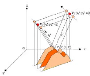
(3) コンピュータビジョンとイメージメディア 134−5 (2002. 9. 12). image number j (line number) in the direction where the sensor is moved. Virtual projective plane coordinate system (u, v) is a right hand coordinate system where the distance in the range direction corresponds to u axis and the distance in the azimuth direction corresponds to v axis. Object space coordinate system (x, y, z) is a right hand coordinate system where x axis and y axis are parallel to u axis and v axis respectively (Fig.2).. Fig. 3. A spatial series of underwater acoustic images taken at different viewpoints. the formula of spatial relation as following: Fig.2. Geometric model of underwater acoustic image. ri2 = (xi - x)2 + ( yi - y)2 + ( zi - z)2 ,. The correspondence of image point P’ (u, v) and object P (x, y, z) is ideally given by the following expression.. i = 1, 2, …, n.. u v. =. √ ̄ ̄ ̄ ̄ ̄ ̄ ̄ (x – x0)2 + (z– z0)2 y. +. u0 v0. , (2.1). where, y = y0. C. Basic Idea Based on Multi-views Model As described above, the range information is included in the underwater acoustic image. But using one image we just can obtain the slant range from the sensor to the object but not synthesize the position of the object in 3-D space. Because, as we know, simple sonar consists of one cylindrical source that creates a conic acoustic beam pattern that is symmetric around the axis of the source. This type of sonar will measure the range to the first surface it encounters within the cone and the intensity or echo of the return; however, the position of the surface cannot be localized within the cone. Since this reason, the range information was ignored and not considered to reconstruct 3-D information. In this paper, our basic idea is that, using a spatial series of underwater acoustic images overlapped each other, which were taken at different “viewpoints” when the side-scan sonar tracked along parallel course (Fig. 3), we can estimate their positions in 3-D space according to. (2.2). Here, i is the number of viewpoint, (xi, yi, z i) is the position of viewpoint i, and (x, y, z) is the position of the point on the object surface, ri is slant range from the viewpoint i to the point on the object surface. Since the side-scan sonar tracked along parallel course, we can consider the different (usually two) viewpoints as in same plane, so formula (2.2) can be rewritten to: ri2 = (xi - x)2 + (zi - z)2,. (2.3). i = 1, 2, …, n.. There is a problem remained above how to synthesize the points between the different images as same point in the real 3-D space. This is referred to as the matching problem in computer vision, which is considered a challlenging task due to its difficulty. Contributing factors to this difficulty include the lack of image texture, object occlusion, and acquisition noise, which yield frequently in real imaging applications [13]. In order to solve such problems, there are a lot of methods developed over the last decades. Generally, they can be classified to two types, area-based and feature-based [14-16]. In this work, we developed a new method, Multi-step Gray-level Projective Matching with GPS Positioning, which bases on combining the positioning technology of GPS and the matching. 3 −35−.
(4) コンピュータビジョンとイメージメディア 134−5 (2002. 9. 12). technology of the computer vision.. III. SENSOR TRACKING AND FRAME DETERMINATION OF CORRESPONDING SUB-IMAGES A. Sensor Tracking Sensor tracking is to get a set of position data of side-scan sonar in the real 3-D space. For horizontal tracking, a set of synthesized GPS data are used. As the GPS is not directly located on the side-scan sonar (Fig. 4), it is possible that geometric distortions caused by movement of the sensor that do not rely on onboard navigation measurements [17]. In this work, an experiential value is set as initial layback, and then corrected by the motion estimation method introduced later.. In order to match multi-view images, the frame of corresponding sub-image should be determined. Under the frame, corresponding sub-image in each image can be extracted, and all corresponding subimages can be registered each other to find corresponding points. First, as the maximum slant range of side-scan sonar should be set up beforehand and the average depth from side-scan sonar to the bottom has been known, the maximum ground range that is covered by the side-scan sonar can be calculated according to the geometric model of underwater acoustic image. Next, the slant range image is projected to the ground range, which the projected image is called “ground range image”. Second, as we know, the range direction is orthogonal to azimuth direction, so that the ground range image can be registered to a global 2-D map along the normal direction of the wake of side-scan sonar (Fig. 6. a). Similarly, another overlapped underwater acoustic image can be registered too. Third, the frame of corresponding sub-image overlapped each other can be determined and the corresponding sub-images can be extracted (Fig. 6. b).. Fig.4. Relative position between sonar and GPS. For vertical tracking, as we know, for each impulse, the reverberated signals from the seabed right under side-scan sonar are generally the fastest. It means first bigger change of gray-level from centerline to both sides on the image will be measured. A running mean filter is used to reduce noise and an average depth is considered as the plane of seabed (fig. 5).. (a). (b). Fig.6. Frame determination of corresponding subimages: (a) Register to a global 2-D map; (b) Frame of corresponding sub-images. IV. MULTI-STEP GRAY-LEVEL PROJECTIVE MATCHING. (a). (b). Fig.5. Tracking for vertical position of sonar: (a) First bigger change of gray-level from centerline to both sides; (b) Depth and average depth. B. Frame Determination of Corresponding Sub-images. A. Motion Estimation in Azimuth Direction As explained above, the misalignment of horizontal position exists between the different images. It is difficult to directly synthesize the GPS data and the side-scan data. About motion estimation, a lot of approaches have been developed over the last decades in the several relative fields such as stereovision and analysis of image sequences [18-23]. In many cases the input underwater acoustic images are strongly corrupted by speckle noise [1, 2]. Therefore, we study methods using gray-level projection to reduce the noise effect.. 4 −36−.
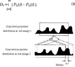
(5) コンピュータビジョンとイメージメディア 134−5 (2002. 9. 12). First, all gray-level of the pixels along the range direction are projected to the azimuth direction over two images. Let gray-level of the pixel (i, j) and the range width in image f1 be G1 (i, j) and w 1, respectively. The projective distribution of number i is defined as 1 w1 PY1 (i) = ∑ G1 (i, j), w1. projective distribution both along the azimuth direction and the range direction in the each zone again. We select the cross points as the feature points where there are bigger changes of the projective distribution (Fig. 8).. (4.1). i=1. same way for image f2, the projective distribution of number i is defined as 1 w2 PY2 (i) = ∑ G2 (i, j). w2. (4.2) Fig. 8. Extraction of feature points. i=1. Next, Getting a center part where larger motion estimation may be looked for from the projective distribution for each image, let PY1 be as reference, shifting PY2, compare these two projective distributions (Fig. 7). The motion estimation will be found when the difference between these two projective distributions is the smallest. The difference degree DY is defined as w DY = ∑ | PY1(i) – PY2(i) |. i=1. (4.3). C. Mutual Matching After selected the feature points, we match the feature points over the different images. Since the occlusion problem exists in underwater acoustic imaging, we use a mutual matching between the different images [24]. First, let one feature point in image f1 is as reference; search the corresponding point in the image f2. Next, let the feature point found above step in image f2 is as reference, search the corresponding point in the image f 1. Just only mutual matching is successful, the points are considered as confident correspondent ones (Fig. 9).. Fig. 9. Mutual matching. Fig.7. Motion estimation using gray-level projective distribution. V. EXPERIMENT B. Extraction of Feature Points After the motion is detected and corrected in the azimuth direction, the search area of corresponding points over two images can be limited in a smaller area along the azimuth direction to reduce the computational burden of matching. So, first, we separate the sub-images into several zones along the azimuth direction, and then use the gray-level. To validate our method for 3-D reconstruction of seabed, we have carried out an experiment with EdgeTech’s DF1000 side-scan sonar and JRC’s DGPS200 GPS in Seto inland sea, Japan, and the result shows the method is valid. Fig.10 is a pair of input underwater acoustic images taken along a set of parallel courses (see. −37− 5.
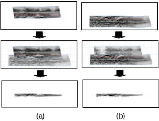
(6) コンピュータビジョンとイメージメディア 134−5 (2002. 9. 12). the selected area in Fig.11).. Image1. Image2. Fig.10. A pair of input underwater acoustic images. Fig.11 and 12 show the tracking results of sidescan sonar. In Fig.11, a horizontal tracking is presented, which a set of synthesized GPS data was used in processing. In Fig.12, a pair of vertical tracking is presented using the depth estimation method described in Section 3 A.. (a). (b). Fig. 13. Process for extraction of corresponding sub-images: (a) Image 1; (b) Image 2. Fig.14 shows a result of motion estimation and correction in azimuth direction using gray-level projective distribution, which was introduced in Section 4 A.. Selected area (a). (b). Fig. 14. Result of motion estimation and correction in azimuth direction: (a) Before correction; (b) After correction. Fig.11. Tracking of side-scan sonar. Fig.15 presents a process for extraction of feature points, using the method introduced in Section 4 B. Here, feature point search was limited a smaller to improve the effect of gray-level projective distribution in range direction. (a). (b) Fig.12. Depth estimation of side-scan sonar: (a) Course 1; (b) Course 2 Fig. 15. Process for extraction of feature points. Fig.13 shows a process for extraction of corresponding sub-images using the method described in Section 3 B.. Fig.16 shows a result of feature points matching over two images, using the method introduced in Section 4 C.. 6 −38−.
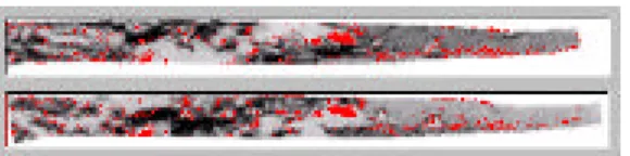
(7) コンピュータビジョンとイメージメディア 134−5 (2002. 9. 12). Fig. 16. Result of mutual matching. Finally, the 3-D structure of seabed was estimated by using a pair of range data sets obtained by matching feature points over two images. Fig.17 shows the result.. Fig.17. The 3-D reconstruction of seabed. VI. CONCLUSIONS In this paper, we have presented an original approach to the 3-D reconstruction problem from the underwater acoustic images. It is based on a multi-view method, which uses a combination of the GPS positioning and the image matching technology. The GPS positioning component of the technique tracks the side-scan sonar and determine the corresponding sub-image between different images according to the geometric model of underwater acoustic image. The image matching part of the techniques matches the corresponding points between the each corresponding sub-image using the method of multi-step gray-level projective matching. The proposed scheme appears as an appealing alternative to the 3-D reconstruction approaches for underwater acoustic image using shape from shading or multi-views techniques.. REFERENCES [1] M. Nignotte, C. Collet, P. Perez, and P. Bouthemy, “Markov random field and fuzzy. logic modeling in sonar imagery: application to the classification of underwater floor,” Computer Vision and Image Understanding, vol. 79, pp. 4 -24, July 2000. [2] Xiaoou Tang and W. Kenneth Stewart, “Optical and sonar image classification: Wavelet packet transform vs Fourier transform,” Computer Vision and Image Under-standing, vol. 79, pp. 25-46, July 2000. [3] Y. Lu and M. Oshima, “Study on 3-D reconstruction from underwater acoustic Images”, Proc. the 2000 Conference of Marine Acoustic Academy, Japan, pp. 43-46, June 2000. [4] John P. Fish and H. Arnold Carr, Sound Reflections, Lower Cape Publishing, Orleans, MA, 2001. [5] M. Jiang, W. Stewart, and M. Marra, “Segmentation of seafloor side-scan imagery using Markov random fields and neural networks,” Proc. OCEANS, Victoria, 1993, vol. 3, pp. 456-461. [6] Freddy Pohner, “Technology for mapping and inspection of the ocean seafloor,” Korean / Norwegian Workshop on Ocean Mining, pp. 3146, Seoul, 1997. [7] R. H. Hansen and P. A. Andersen, “The application of real time 3D acoustical imaging,” Oceans Conference Record (IEEE), 1998, vol. 2 pp. 738-741. [8] P. N. Denbigh, “Swath bathymetric: Principles of operation and analysis of errors,” IEEE Journal of Ocean Engineering, vol. 14, pp. 289298, October, 1989. [9] A. E. Johnson and M. Herbert, “Three dimensional map generation from side-scan sonar images,” Journal of Energy resources Technology, Transactions of the ASMET 1990, vol. 112, pp. 96-102. [10] A. E. Johnson and M. Herbert, “Seafloor map generation for autonomous underwater vehicle navigation,” Autonomous Robots, vol. 3, 2-3, (Jun-Jul 1996), pp. 145-168. [11] B. Zerr and B. Stage, “Three-dimensional reconstruction of underwater objects from sequence of sonar images,” Proc. International conference on Image processing, vol. 3, pp. 927930, September 1996. [12] E. Dura, D. Lane, and J. Bell, “Automatic 3D reconstruction of mine geometries using multiple side-scan sonar images,” Goats 2000 Conference, (Aug. 2001). [13] A. Arsenio and J. Marques, “Performance analysis and characterization of matching algorithms,” Proc. The International Symposium on intelligent Robotic System, Stockholm,. 7 −39−.
(8) コンピュータビジョンとイメージメディア 134−5 (2002. 9. 12). Sweden, July 1997. [14] Takeo Kanade and Masatoshi Okutomi, “A stereo matching algorithm with an adaptive window: Theory and experiment,” IEEE trans. PAMI, vol. 16, no. 9, pp. 920-932, 1994. [15] Umesh R. Dhond and J. K. Aggarwal, “Stereo matching in the presence of narrow occluding objects using dynamic disparity search,” IEEE Trans. PAMI, vol. 17, no. 7, pp. 719-724, July 1995. [16] P. Fua and Y. G. Leclerc, “Object-centered surface reconstruction: Combining multi-image stereo and shading,” International Journal of Computer Vision, vol. 16, pp. 35-56, 1995. [17] D. T. Cobra, A. V. Oppenheim, and J. S. Jaffe, “Geometric distortions in side-scan sonar images: A procedure for their estimation and correction,” IEEE J. Oceanic Engineering, 17 (3), pp. 252-268, 1992. [18] T. Huang and A. Netravali, “Motion and structure from feature correspondences: A review,” Proc. IEEE, vol. 82, No. 2, pp. 252268, 1994. [19] Z. Zhang, “Estimating motion and structure from correspondences of line segments between two projective images,” IEEE Trans., On PAMI, vol. 17, no. 12, pp. 1129-1139, 1995. [20] N. Ohta, “Optimal structure-from-motion algorithm for optical flow,” IEICE Trans., vol. E78-D, no. 12, pp. 1559-1566, 1995. [21] R. Szeliski and H. Shum, “Motion estimation with quad tree splines”, IEEE Trans., On PAMI, vol. 18, no. 12, pp. 1199-1210, 1996. [22] F. Chen and D. Suter, “Elastic spline models for human cardiac motion estimation,” Proc. IEEE Nonrigid and Articulated Motion Workshop, pp. 120-127, 1997. [23] N. Gracias and J. Santos-Victor, “Underwater video mosaic as visual navigation map,” Computer Vision and Image understanding, vol. 79, pp. 66-91, 2000. [24] Harlyn Baker, Robert Bolles and John Woodfill, “Real-time stereo and motion integration for navigation,” Proc. Image Understanding Workshop, 1994.. −40− 8 E.
(9)
図

+2
関連したドキュメント
しかしながら,式 (8) の Courant 条件による時間増分
一方,著者らは,コンクリート構造物に穿孔した 小径のドリル孔に専用の内視鏡(以下,構造物検査
2000 個, 2500 個, 4000 個, 4653 個)つないだ 8 種類 の時間 Kripke 構造を用いて実験を行った.また,三つ
玄達瀬近くの海深- 270 mより越前焼大甕を引き揚
The application of steelmaking slag to the dredged material improved the hardness of the dredged material by forming calcium-silicate-hydrooxide (CSH), which strongly affected
「Skydio 2+ TM 」「Skydio X2 TM 」で撮影した映像をリアルタイムに多拠点の遠隔地から確認できる映像伝送サービ
Figure 3 shows the graph of the solution to the optimal- ity system, showing propagation of CD4+ T cells, infected CD4+ T cells, reverse transcriptase inhibitor and a protease
The approach based on the strangeness index includes un- determined solution components but requires a number of constant rank conditions, whereas the approach based on
