Multi-server Queue with Job Service Time Depending on a Background Process

全文

(1)Multi-server Queue with Job Service Time Depending on a Background Process Tomoyuki Sakata and Shoji Kasahara Graduate School of Information Science, Nara Institute of Science and Technology Takayama 8916-5, Ikoma, Nara 6300192, Japan {sakata.tomoyuki.so7, kasahara}@is.naist.jp. Abstract. One of approaches to reducing energy consumption in a data center is to power down a group of servers. In this paper, we consider a power management scheme for distributed parallel processing over clusters of servers, where part of servers in each cluster are turned off in power-saving mode. We model the system as a multi-server queue in which the service time of a job depends on the state of a background process at the beginning of the job service. We analyze the joint distribution of the number of jobs in system and the state of the background process, deriving the mean job-response time and mean amount of energy consumption. In numerical examples, we investigate how the mean job-response time and energy consumption are affected by energy saving level and the number of clusters.. 1. Introduction. Recently, cloud computing has been attracted considerable attention, and various kinds of computing services such as virtual machines and MapReduce software framework are provided by data centers. A data center contains a large number of server machines, resulting in high energy consumption. With the increase in cloud computing demand, the number of data centers is growing rapidly, and the amount of energy consumption for data centers is extremely huge. Therefore, considerable research efforts have been devoted to developing schemes which can save energy without degrading job-processing performance. There exist much literature which concerns strategies of efficient energy saving for data centers. A typical scheme for reducing energy consumption in data centers is to manage the power of server machines according to demand for computing resources. In [5], the authors propose a scheme of server-power management for a data center, with which the number of running servers is varied according to the number of jobs in system. If the number of waiting jobs exceeds a predefined threshold, all the servers are turned on. If the number of servers busy for job processing are below another threshold, a given number of servers are turned off. In [5], the trade-off between job-waiting time and energy consumption is analyzed by an M/M/c queue with threshold-based on/off control. In [1], the authors propose Berkeley Energy Efficient MapReduce (BEEMR), an efficient power management scheduling for MapReduce-type job processing..

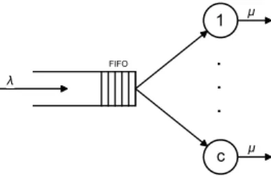
(2) In BEEMR, servers in a data center are divided into two grouping zones, an interactive zone and a batch zone. The servers in the interactive zone are always turned on and serve small-sized jobs. On the other hand, the servers in the batch zone process huge-sized jobs that are insensitive to the response time. BEEMR controls the power of servers in the batch zone so that the amount of power consumption is reduced. The authors in [1] investigate the performance of BEEMR by simulation and on-site practical experiments. In [2], the performance of BEEMR is investigated by queueing theoretical approach. In this paper, we consider a power-management scheme for data centers with server clusters. We focus on a data center accommodating a large number of server clusters, each of which consists of several server machines, providing parallel distributed computing service. The data center alternates two poweroperation modes: normal-operation and power-saving. The power of server machines is managed in a cluster-based manner. When the data center is in normaloperation mode, all the servers of all clusters are powered on. When the data center switches to power-saving mode, a part of servers in each cluster are powered off after completing the existing job. In both operation modes, a job is served by a cluster according to processor sharing discipline. Therefore, the service rate of a cluster in power-saving mode is smaller than that in normal mode. In order to investigate the performance of the cluster-based power management scheme, we model the data center as a multi-server queueing system with job service depending on the state of a background process. Here, a server of the queueing model corresponds to a cluster of machines in the data center. The service time of a job depends on the state of the background process at the beginning of the job’s service. We construct a trivariate continuous-time Markov chain for the system, deriving the steady-state probability vector by matrix geometric method. We consider the mean job-response time and mean amount of energy consumption as performance measures, and investigate how the performance measures are affected by system parameters such as the number of clusters and the parameter indicating energy-saving level. This paper is organized as follows. In Sect. 2, we describe the queueing model considered in this paper, and analyze the steady-state distribution by matrix analytic method in Sect. 3. Numerical examples are shown in Sect. 4, and finally in Sect. 5 our conclusion is presented.. 2. Queueing Model. Figure 1 shows the model considered here. We assume that the number of servers is c, and that the buffer capacity is infinite. Jobs arrive at the system according to a Poisson process with rate λ. The service time of a job depends on the state of a background process when the job service starts. The background process is continuous-time Markov chain with two states, Slow (S) and Fast (F ), independent of the arrival process. The state S describes the power-saving mode in which a part of worker machines are turned off for energy saving, and hence the resulting service rate of a server is low. When the state of the background.

(3) Fig. 1. Queueing model.. process is F , on the other hand, all the worker machines composing a server are turned on and the resulting service rate of the server is greater than that in state S. The state-transition rate from S to F and that from F to S is given by αS and αF , respectively. When a job enters a server for its service, its service time depends on the state of the background process. If the background process is in state S (resp. F ) at the service initiation point, the service time of the job follows an exponential distribution with rate µS (resp. µF ). In the following, µS < µF . We also assume that when the background process switches from S to F (and vice verca), the service rate of the existing job remains the same as that at its service initiation point. Hereafter, a job served with rate µS and that with rate µF are called S job and F job, respectively.. 3. Analysis. We define N (t) as the number of jobs in the system at time t. Let S(t) and F (t) denote the numbers of S jobs and F jobs at t, respectively. We denote J(t) (∈ {S, F }) as the state of the background process at t. F (t) can be expressed with N (t) and S(t) by F (t) = min(N (t), c) − S(t). From the assumptions, {(N (t), S(t), J(t)) : t ≥ 0} is a trivariate continuous-time Markov chain with state space IF, where IF is given by IF = IN ∪ {0} × {0, 1, . . . , c} × {S, F }. Let Q denote the infinitesimal generator of the Markov chain {N (t), S(t), J(t) : t ≥ 0}, whose states are arranged in lexicographic order. Then, Q is given by   B B0 O O O O · · ·  B1 A1 A0 O O O · · ·      Q =  O A2 A1 A0 O O · · ·  . (1)  O O A2 A1 A0 O · · ·    .. .. .. . . ..

(4) In what follows, we describe the details of block matrices B, B0 , B1 , A0 , A1 , and A2 in (1). Hereafter, i is an integer such that the inequality k(k + 1) < i ≤ (k + 1)(k + 2) holds for any k ∈ [0, c], and [x] is the largest integer not greater than x. (a) c(c + 1) × c(c + 1) matrix B (i) For odd i,  αS ,      λ,    d(k + 1, i + 1) µ , F [B]ij =  −d(k, i − 1) µ , S      −αS − λ − d(k + 1, i + 1) µF + d(k, i − 1) µS ,    0, where d(k, i) = (ii) For even i,. [B]ij. k(k + 1) − i . 2.   αF ,    λ,    d(k + 1, i) µ , F =  −d(k, i − 2)µ S,     −αF − λ − d(k + 1, i) µF + d(k, i − 2)µS ,    0,. (b) c(c + 1) × 2(c + 1) matrix B0 (i) For odd i, [B0 ]ij. { λ, = 0,. j = i − c(c − 1) + 2 and j ̸= 1, otherwise.. (ii) For even i, [B0 ]ij =. { λ, 0,. j = i − c(c − 1), otherwise.. (c) 2(c + 1) × c(c + 1) matrix B1. [B1 ]ij. j = i + 1, j = i + 2k + 4, j = i − 2k, j = i − 2k − 2, j = i, otherwise,. ]) [ ( i−1   µF , c −   2   [ ] = i−1  µS ,    2   0,. j = i + c(c − 1), j = i + c(c − 1) − 2, otherwise.. j = i − 1, j = i + 2k + 2, j = i − 2k, j = i − 2k − 2, j = i, otherwise..

(5) (d) 2(c + 1) × 2(c + 1) matrix A0 [A0 ]ij. { λ, = 0,. j = i, j ̸= i.. (e) 2(c + 1) × 2(c + 1) matrix A1 (i) For odd i,. [A1 ]ij.   αS ,   [ ] ( [ ])  i−1 i−1 = −αS − λ − µS − c − µF ,  2 2   0,. j = i + 1, j = i, otherwise.. (ii) For even i,. [A1 ]ij.   αF ,   [ ] ( [ ])  i−1 i−1 µS − c − µF , = −αF − λ −  2 2   0,. j = i − 1, j = i, otherwise.. (f) 2(c + 1) × 2(c + 1) matrix A2 (i) For odd i,. [A2 ]ij.  i−1   µS ,    ( 2 ) i−1 = c − µF ,    2   0,. j = i, j = i + 2, otherwise.. (ii) For even i,. [A2 ]ij. ) ( i−2   c− µF ,   2   = i−2   µS ,     2 0,. j = i, j = i − 2, otherwise.. We define the steady-state probability as π(i, j, k) = lim Pr{N (t) = i, S(t) = j, J(t) = k}, t→∞. (i, j, k) ∈ IF.. We also define the following notations. π−1 = (π(0, 0, S), π(0, 0, F ), π(1, 0, S), π(1, 0, F ), π(1, 1, S), π(1, 1, F ), . . . , π(c − 1, 0, S), π(c − 1, 0, F ), π(c − 1, 1, S), π(c − 1, 1, F ), . . . , π(c − 1, c − 1, S), π(c − 1, c − 1, F )), πi = (π(c + i, 0, S), π(c + i, 0, F ), π(c + i, 1, S), π(c + i, 1, F ), . . . , π(c + i, c, S), π(c + i, c, F )),. i ≥ 0..

(6) Let π = (π−1 , π0 , π1 , . . .). π is the steady-state probability vector which satisfies πQ = 0 and πe = 1. From (1), this continuous-time Markov chain is a quasi birth-and-death process. The steady-state probability vector π can be calculated by matrix-analytic method [3]. In terms of the system stability, we have the following theorem. Theorem 1. ([4], p. 411, (9.36)) We assume that 2(c + 1) dimensional square matrix A = A0 + A1 + A2 satisfies πA A = 0 and πA e1 = 1. Then, the stability condition for the system is πA A0 e1 < πA A2 e1 . In our case, we can conjecture the following stability condition. ) ( 2 + αS µF + αF µS cµS µF αS2 + 2αS αF + αF λ< . (αS + αF )(αS µS + αF µF + µS µF ). (2). Finally, we consider two performance measures: the mean job-response time and mean amount of energy consumption. Let a denote the 1 × c(c + 1) vector whose ith element is given by [a]i = k,. k(k + 1) < i ≤ (k + 1)(k + 2),. for k = 0, 1, 2, . . . , c − 1. The mean number of jobs in system is then given by E[L] = aπ−1 +. ∞ ∑ (c + i)πi e1 .. (3). i=0. Using Little’s law, the mean job-response time E[T ] is given by E[T ] = E[L]/λ. Let E denote the mean amount of energy consumption per unit time. E can be expressed as ∑ π(i, j, k){jµS + min(c − j, i − j)µF + max(0, c − i)κµk }, E= (i,j,k)∈IF. where κ is the ratio of the amount of energy consumption of a single idle server to that of a single busy server.. 4. Numerical Examples. We define ζ as ζ = µS /µF . ζ is related to the ratio of the service rate of powersaving mode to that of normal-operation mode. A large ζ indicates that the number of worker machines turned off in power-saving mode is small. In other words, a large ζ implies a small amount of energy saving for the system. Note that when the system is in power-saving mode, all servers keep running for ζ = 1, whereas all the servers are turned off for ζ = 0. In the following, we set κ = 170/240. We only consider the case of λ = 12 and αS = αF = 1 due to page limitation..

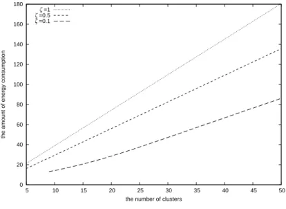
(7) 2.5. ζ =1 ζ =0.5 ζ =0.1. mean job response time. 2. 1.5. 1. 0.5. 0 5. 10. 15. 20. 25 30 the number of clusters. 35. 40. 45. 50. Fig. 2. c vs. E[T ].. Figure 2 illustrates the mean job-response time E[T ]. The horizontal axis is the number of clusters c, and E[T ]’s for ζ = 0.1, 0.5, 1 are plotted. Note that ζ = 1 under αS = αF corresponds to the case of an M/M/c with service rate µF . We observe from the figure that when c increases, E[T ]’s for the three cases decrease and converge to some constants. We also observe that E[T ] increases with the decrease in ζ. A remarkable point here is that the discrepancy between ζ = 1 and ζ = 0.5 is significantly smaller than that between ζ = 1 and ζ = 0.1. When ζ = 0.5, a half of servers in a cluster are powered off in power-saving mode. This figure shows that energy-saving level of ζ = 0.5 does not degrade the job-response time. Figure 3 represents E against the number of clusters c. In this figure, the amount of energy consumption increases linearly for any ζ, as expected. We also observe that E for ζ = 1 is the largest for any c, and that E becomes small with the decrease in ζ. Note that the power-saving level of ζ = 0.5 effectively reduces E even for a small c. This result suggests that the power-saving level of ζ = 0.5 is effective both for reducing the energy consumption and for keeping the job-response time small.. 5. Conclusion. In this paper, we considered a queueing model for data centers with BEEMR-like energy-saving management mechanism. We modeled a data center as a multipleserver queue with job service depending on a background process. Using matrixanalytic method, we derived the joint distribution of the number of jobs in system and the state of the background process, yielding the mean job-response time.

(8) 180. ζ =1 ζ =0.5 ζ =0.1. 160. the amount of energy consumption. 140. 120. 100. 80. 60. 40. 20. 0 5. 10. 15. 20. 25 30 the number of clusters. 35. 40. 45. 50. Fig. 3. c vs. E.. and mean amount of energy consumption as performance measures. Numerical examples showed that turning a half of servers in a cluster is effective for keeping the mean job-response time small. We also observed that the amount of energy consumption grows linearly with the increase in the number of clusters. We can conclude that turning part of servers in a cluster off at power-saving mode is effective enough for saving energy consumption. In addition, a small job-response time can be achieved even with a small number of clusters.. References 1. Y, Chen, S, Alspaugh, D, Borthakur and R, Katz: Energy Efficiency for Large-Scale MapReduce Workloads with Significant Interactive Analysis. Proc. The European Professional Society on Computer Systems April. 2012, 43–56 (2012) 2. M, Kato, H, Masuyama, S, Kasahara, and Y, Takahashi: Performance Analysis of Energy-Saving Server Scheduling Mechanism for Large-Scale Data Centers. Proc. The 9th International Conference on Queueing Theory and Network Applications (QTNA2014), Bellingham, USA, August. 2014, 28–35, 18–21 (2014) 3. G, Latouche and V, Ramaswami: Introduction to Matrix Analytic Methods in Stochastic Modeling. ASA-SIAM, (1999) 4. R, Nelson: Probability, Stochastic Processes, and Queueing Theory. Springer Verlag (2000) 5. C, Schwarts, R, Pries and P, Tran-Gia: A Queuing Analysis of an Energy-Saving Mechanism in Data Centers. Proc. International Conference on Information Networking 2012, February. 2012, 70–75 (2012).

(9)