鹿児島大学リポジトリ

(1)

Design of Linear Stationary Stochastic Estimators

●

in Relation to H｡｡ Estimation Technique

Seiichi Nakamori : (Received 30 September, 1998)

91

Abstract

This paper designs the fixed-point smoother and filter suitable for estimating the

wide-● wide-● wide-●

sense stationary stochastic signal in relation to the 〃∞ estimation approach in

continuous-●

time systems. Performance measure for the design of the estimators is newly introduced by ● ●

referring to that of the infinite-horizon H^ estimation problem in the Krein spaces [1],[2]. At first, we propose the estimation algorithms using the covariance information in linear

con-●

tinuous wide-sense stationary stochastic systems. Secondly, to improve the estimation accu-racy of the recursive least-squares (RLS) estimators [3] using the covariance information, the suboptimal fixed-point smoother and filter using the covariance information are proposed.

●

● ●

Finally, the recursive比Iike fixed-point smoother and filter using the state-space parameters

are derived from those using the covariance information in a unified manner in linear con-tinuous wide-sense stationary stochastic systems.

1. Introduction

Recently, by use of the state-space parameters, the H｡｡ and its related estimation tech-niques [l],[2],[4]-[8] have attracted great attention in the deterministic and stochastic estima-tion methods of signal. Incidentally, as an alternative approach to the leasトsquares estimaestima-tion

problem based on the state-space model, the recursive Wiener fixed-point smoother and filter

using the covariance information of the signal and the observation noise are developed in ● ●

linear continuous stochastic systems [3].

The performance criterion concerned with the 〃∞ estimation problem is formulated in

the deterministic manner by nature. The problem formulation in the finite-horizon and inn-nite-horizon H｡｡ estimation problems is limited within deterministic representations and would

not fit to the estimation in linear stationary stochastic systems. In [1],[2] the deterministic //ォ technique in the Krein spaces is developed. In the H｡｡ estimation problem [1],[2], the

perfor-* Department of Technology, Faculty of Education, Kagoshima University, 1 -20-6, Kohnmoto, Kagoshima 890-0065, Japan

(2)

mance criterion is represented as Eq.(4) in section 2. In the H2 estimation problem, the value of γま(see Eq.(4)) is set to …[l],[2],[4]-[8]. Consequently, the estimation accuracy of the //ォ estimator is superior to the H2 estimator. Taking into account of these aspects, we introduce

●

the performance criterion newly. We examine to design the estimators, which correspond to

the 〃∞ estimator, to improve the estimation accuracy in comparison with the RLS Wiener

●

estimators [3], which correspond to the Hi estimator in the H^ estimation problem, in linear wide-sense stationary stochastic systems [9]. At first, in section 2, the stochastic signal esti-mation problem is introduced for the estiesti-mation of the wide-sense stationary signal. Based on

●

the current performance criterion (see Eq.(5)), as in the deterministic //｡｡ estimation tech-mque [1],【2], we obtain the observation equation in the wide-sense stationary stochastic sys-tems. Assuming that the observation equation is given, we consider the linear least-squares

● ●

estimation problem using the covariance information in wide-sense stationary stochastic sys-●

terns.

In the observed values, an artificial observed value z (t) (see Eq.(9)) is included. In [Theo-rem l], by use of the covariance information of the signal and the observation noise, recursive algorithms for the fixed-point smoothing and filtering estimates of the signal z(t) (see Eq.(8))

are proposed. In [Theorem 2], based on the algorithms of [Theorem l], recursive Wiener

fixed-point smoother and filter using the covariance information are proposed. Recursive Wiener fixed-point smoother and filter for the signal z(t) use the system matrix F9 the obser-vation matrix H (see Eq.(8)), the crosscovariance function Kxy(t,T) of the state variable x(t) with observed value y(T), the crossvariance function Kxy(T, T), the variance S of the observa-tion noise (see Eq.(lO)) and the observed value y(T) (see Eq.(9)). From the estimaobserva-tion equa-tions in [Theorem 2], [Theorem 3] formulates the algorithms using the covariance informa-tion for the fixed-point smoothing estimates z¥(t,T) and z2(t,T) at the fixed point t and the filtering estimates z¥(TyT) and z¥(T,T) for the components z¥(t) and z2(t) of the signal vector

z(t). According to the derivation of the 〃∞ suboptimal estimators [2], we propose in

[Theo-rem 4] the recursive suboptimal fixed-point smoother and filter using the covariance infor-mation by setting吉(T) - z2(T, T) in the estiinfor-mation algorithms of [Theorem 3]. Here, the esti-mation algorithms of [Theorem 4] necessitate the inforesti-mation of the observation matrices C and L (see Eq.(8)), the system matrix F, the autocovariance function Kx(t,T) of the state vari-able x(t), the autovariance function Kx(T, T), the crosscovariance function Kxyx(t> T) of the state variable x(t) with the observed value yi(T)9 the crossvariance function Kxyx(T, T), y (see Eq.(5)) and the observed value y¥(T)(sec Eq.(2)). For y2=-, the fixed-point smoothing and filtering

(3)

Design of Linear Stationary Stochastic Estimators in Relation to H∞ Estimation Technique 93

smoothing and filtering estimates in [3]. [Theorem 5] shows the optimal fixed-point smooth-ing and filtersmooth-ing algorithms ussmooth-ing the state-space parameters. They are derived from the

esti-● esti-● esti-●

mation algorithms of [Theorem 3] using the covariance information. The algorithms of [Theo-rem 5] uses the system matrix F, the observation matrices C and L, the input matrix Z?(see Eq.(l)), Y, the observed values y¥(T) and z(T). In [Theorem 6], assuming that the observed value z(T) of zi(T) introduced artificially is equal to z2(T,T) in the estimation equations of [Theorem 5], we propose the suboptimal algorithms using the state-space parameters for the fixed-point smoothing and filtering estimates of z¥(t) and zi(t). The suboptimal filtering algo-rithm using the state-space parameters in [Theorem 6] is same as that based on the game theory approach [5] in linear continuous stochastic systems. For y2=oo9 the suboptimal filter is reduced to the Kalman filter. The suboptimal fixed-point smoothing algorithm in [Theorem 6] is proposed for the first time in this context.

2. Problem Formulation

Let the linear time-invariant state-space model for the state variable x(t) be given by

dx(t)

dt = Fx(t)+Bu(t),x(O) = xQ,

E[u(t)u'(s)]- no S(t-S).

(1)

Here,x(7)∈K ,u(t) ∈Rt.F represents the system matrix and B the input matrix for u(t). Let z¥(t)

represent a signal expressed by z¥(t)=Cx(t). We assume that the signal z¥(t) is observed with

additive white Gaussian noise vi何.

yi(t)=Zi(t)+vl(t), zi(t)-Cx(t), E¥vAt)v[ (5)]=RS(t-s) (2)

Here, y¥(t) represents the observed value and C m by n observation matrix. We assume that

v¥(t) and u(t) are uncorrelated. We also assume that (F,C) is observable and xq is a random

variable with the mean zero and the variance Qo.

Let a signal zi{t) be represented by

z2(t)=Lx(t) , (3)

where L is r by n vector.

Let Li¥Q,T¥ denote the usual Hilbert space of square integrable functions. In the

finite-horizon H｡｡ estimation problem, the estimators are designed so as to achieve the following

● performance measure [2] :

(4)

Sup xoMn∈L2,*(O,vi (f)∈LJ2 千 ∫(z(t)- Lx(t))'(z(t)- Lx(t))dt 0 rr JA-I x｡Q｡x｡+JuT(t)u(t)dt+JvT x(t)vx(t)dt O0 <ri (4) ′､

Here,?(rJ is the artificial observed value for zi(t) and Qo is a definite weighting matrix. Qo

reflects a priori knowledge as to how close x(0) is to its initial guess. We assume that initial

guess ofx(0) is zero without loss of generality. For the case of T=-, the performance criterion (4) is concerned with the infinite-horizon H^ estimation problem. In the H^ estimation prob-lem, we make no assumption of the nature of the noises disturbances u(t) and v¥(t) (e.g. normally distributed, uncorrelated, etc.) and consider to estimate z2(t)=Lx(t). It is clear that the problem formulation for the H^ estimation problem would not fit to treat the estimation problem which assumes the priori statistics for 〟何and vi何in (1) and (2) in wide-sense

stationary stochastic systems [9].

●

In this paper, instead of the H^ estimation problem, we consider to estimate the signal z2(t)=Lx(t) in the wide-sense stationary stochastic systems by taking into account of the sta-tistical properties for u(t) and v¥(t) in (1) and (2). Along with this idea, we newly introduce the

performance criterion represented by

E[(z(t) - Lx(t)Y (z(t) - Lx(t))]

Sup

E[xkQ｡IxQ]+ E[u'(t)Iln'ォ(')]+ E[(y,(t)- Cx(t))'R l(y,(t)- Cx(t))]

<γ (5)

in the wide-sense stationary stochastic systems. Under the criterion of (5), we can now treat the estimation problem for the wide-sense stationary stochastic signal process in which the

●

ergodic process is included. If we introduce the stochastic quantity of the form ●

Jf - ｣U｡C｡ *｡] + E[uT(t)Fl｡ォ(O]+Ei(y¥(0- cx(r))r/? (y,(t)- Cx(t))]

-γ-2E[(z(t) - Lx(t))'(z(t) - Lx(t))l

(6)

we find that the performance criterion (5) in the current stochastic estimation problem is transformed into the relationship satisfying J/> 0. Henceforth,

Jf-E[x' ｡(O)G｡'x｡]+E[u'(t)U｡'u(t)]+ *[rji(o" z{t)CLx(t)R0 0-Y2Ii-i,>i(0" z(040D>o (7)

(5)

Design of Linear Stationary Stochastic Estimators in Relation to H∞ Estimation Technique 95 is obtained in relation to the H^ estimation problem [2]. Let us introduce the vector z(t) which

consists of the signals z¥(t) and zi{t).

z(t)=Hx(t) z z三(｡'H¥l'

zAt)=Cx(t), z2(t)=Lx(t)

Letusalsointroducetheobservationvectory(t) y(t)=y.(o z(t) (8) (9)

which consists ofy¥(t) and the artificial observation z(t) for z2(t). As in the observation equation in the Krein spaces [2], by checking the condition for a minimum of J/> 0, the ob-servation equation in the stationary stochastic continuous-time systems might be written as

y(t)=Hx(t)+v(t), z(t)=Hx(t),

v(0-三ォ)

rTi¥RO

E[v(t)vT(S)¥-ES(t-s),S-I_r2

(10)

The observation equation (10) is analogous to that in the Krein spaces [2] of the linear deter

ministic氏｡ estimation problem. Provided that the observation equation (10) is given, we

consider the stochastic estimation problem in the sense of linear least-squares estimation problem for the fixed-point smoothing and filtering estimates of the signal z(t) and the filter-ing estimate of the state variable x(t).

It should be noted that the performance criterion even in the infinite-horizon H｡｡

estima-tion problem is distinct from the current one given by (5). In the 〃∞ estimaestima-tion problem, we

do not assume a priori knowledge on the variances of the noises 〟( ) and vi(#) with their

uncorrelation property.

Let the fixed-point smoothing estimate x(t, T) of the state variable x(t) be expressed as

千

x(t,T) - Jh{t,sj)y{s)ds (ll)

0

as an integral transformation of the observed data set {y(s), 0≦ S ≦ T}. Here, h(tysj) repre-sents the impulse response function, t" is referred to as the fixed point. The fixed-point

smoothing estimate of the signal z(t) is expressed as z(t,T)=Hx(t,T). We consider the linear

(6)

J - E¥¥x(t)-x(t,Tf (12)

in linear continuous-time stochastic systems, given the observation equation ( 10). Let Kxy(t,s) represent the crosscovariance function of the state variable x(t) with the observed value y(s).

The optimal impulse response function, which minimizes (12), satisfies the Wiener-Hopf

integral equation [3]

r

Kxy(t,s) = ¥ h{t,s', T)E[y(s')yT(s)]ds¥

0

If we substitute (10) into (13), we obtain

rJ

h(t,s,T)E = Kxy(t,s)- ¥ h{t,s',T)HKxy(s',s)ds',

0

(13)

(14)

since the variance of v(t) is S from (10).

In sections 3 and 4, by use of the covariance information of the signal z(t) and the obser-vation noise v(t)9 we present the recursive algorithms for the fixed-point smoothing estimate

z{tj) of the signal z(t) and the filtering estimates z(T,T) of z(T) and x(TyT) ofx(T).

3. Recursive Wiener Smoother and Filter

Let ◎(T,0) represent the state transition matrix of the system matrix F. ◎(t,s), 0 ≦ S ≦ t,

satisfies ∂◎(∫, ∫)

∂J = FQ>(t,s). Let Kz(t,s) represent the autocovariance function of the signal

z(t).Kz(t,s)isexpressedas

Kz(f,s)-Hョ(t,s)Kxy(s,s)l(t-j)+^(r,0*feOォ71(s-1¥

^xyxy^ (15)

where l(t-s) represents the unit step function. [Theorem 1 ] presents the fixed-point smoothing and filtering algorithms of z(t) using the crosscovanance function Kxy(t, T) of the state van-able x(t) with the observed value y(T), the crossvariance function Kxy(T, T), the state transition matrix ◎rT,0), the observation matrix //, the variance 5 0f the observation noise v(t) and the observed value y(T).

【Theorem l】

Let the variance of the initial value xq ofx(t) at t = 0 be Qo > 0. Let the observation equation be given by (10). Then the recursive algorithms for the fixed-point smoothing

esti-mate z(tj) at the fixed point t and the filtering estiesti-mates z(T,T) of z(T) and x(T,T) ofx(T),

which achieve the criterion of (5), consist of (16) -- (24). Here, the estimators use the

crosscovariance function Kxy(t, T) of the state variable x(t) with the observed value y(T), the

crossvariance function Kxy(Ty T), the state-transition matrix ◎(TyO) for the system matrix F,

(7)

the observation matrixガ, the variance三of the observation noise v何and the observed value

y(T).

z(t,T): Fixed-point smoothing estimate of the signal z(t) at the fixed point t.

dz(t, T) ∂r

= Hh(t,T,T)(y(T)- z(T,T))

h(t,T,T)=(KxJt,T)-U(t,T)^T(T,O)HT)E 7-vB-i -xy dU(t, T) ∂r

= h{t,T,T)(KT (T,T)￠T(O,T) - Hョ(T,O)W(T))

U(T,T) = ◎(T,O)W(T) J(T,T)=(◎(0,T)KXJT,T)-W(T) -xy◎T(T,Q)HT)E-l -^P-J(T,T)(K*(T,T)◎T(O,T)-H^(T,O)W(T)), dT W(0)=0

z(T,T): Filtering estimate of the signal z(T). z(T, T)=Hx(T, T)

x(T, T) : Filtering estimate of the state variable x(T). x(T, T)=◎rT, O)e(T)

de(T)

dT = J(T,T)(y(T)- H4>(T,O)e(T)), e(O)- 0

Proof: Let us differentiate (14) with respect to T.

dh(t,s, T) ∂r -h{t, T, T)HKxJ 〟 _ J 0 E i d nJ ㍗ウ r ^d ′ nJ ラ J r t (

闇

∂r (s', s)ds'

If we introduce an auxiliary function q(T,s) which satisfies

q(T,s)E - HKxy(T,s)- j q(T,s')HKxy(s',s)ds',

we obtain the differential equation

(16) 17 18 (19) (20) (21) (22) (25) (26)

(8)

∂坤,∫, r)

cfT = -h(t,T, T)q(T,s)

for h(t,s,T) by comparing (25) with (26). (26) is written as

q(T,s)E = H^(T,0)O(0,s)Kxy(s,s) - i q(T,s')HKxy(s',s)ds'

(27)

(28)

by using the property of the transition matrix ◎(T,s). If we introduce an auxiliary function J(T,s) which satisfies

J(T,s)a - ◎(O,s)Kxy(s,s) - ¥ j{T,s')HKxy{s',s)ds',

we obtain

q(T,s) - H<i>(T,O)J(T,s).

If we differentiate (29) with respect to T, we have

dJ(T, s) aT

E = -J(T,T)HKxy(T,s)- V

T df(T,s') ∂7' HKxv(s',s)ds' -xy

From (28), (30) and (31), we obtain the differential equation dJ(T, s) cfT = -J{T, T)q{T,s) - -J(T, T)〃◎(T,O)J(T, ∫) (29) 30 (31) (32) forthefunctionJ(T,s). Now,thefunctionh(t,T,T)in(27)canbeformulatedasfollows.Ifweputs=Tin(14) andusetheexpressionofKxy(s′,r)forO≦S′≦T,i.e.,HKrv(S',T)-Kl(s',s') xyyxyK◎(T,s')H',we have n h(t,T,T)E-K^(t,T)-fh(t,s',T)HKxy(s',T)ds' 0 -K^Wn-ih(t,s',T)KT xy(s',s')<S>T(T,s')HTds'. Ifweintroduceafunction U(t,T)-jh(t,s',T)K^(s',S')◎T(O,s')ds', weobtain h(t,T,T)-(KxM,T)-U(t,T) -xy◎(T,O)H')≡-1･ Ifwedifferentiate(34)withrespecttoT,anduse(27)and(30),wehave (33) (34) 35

(9)

Design of Linear Stationary Stochastic Estimators in Relation to H∞ Estimation Technique 99 ∂U(t, T) ∂r

- h(t,T,T)KT {T,T)◎ "(0,T)- h(t,T,T)H4>(T,0)J J(T,s')K^y(s',s')◎T(O,s')ds[

(36) If we introduce a function

W(T) -j JiT^'Wlis'J)◎T(O,s')ds',

we obtain the differential equation

dU(t, T)

∂r

=h(t,T,T){KT

xy(T,T)◎(O,T)-HO(T,O)W)(T))

for the function U(t, T).

If we differentiate (37) with respect to T, we have

dwm

J(T,T)KUt,T) xyy◎r(O,T)+f T dJ(T,s') ∂r

^(sv)◎T(O,s')ds'.

Ifwesubstitute(32)into(39)anduse(37),weobtainthedifferentialequation ^11-7(7,T)(KT xy{T,T)ョT(0,T)-Hョ(T,O)W(T)) (37) (38) (39) (40)

for the function W(T). The initial condition on the differential equation (40) at T=O is W(0)=O from(37).

The function J(T,T) in (40) is formulated as follows. If we put s=T in (29) and substitute the expression for Kxy(s',T) into the resultant equation, we have

J(T,T)E - 0(0,T)Kxy(T, T)- J J(T,s')HKxy(s',T)ds'

- <t>(O,T)Kxy(T,T)- j J(T,s')Kl(s',s')◎T(T,s')HTds'.

From(37)and(41),weobtain J(T,T)=(◎(O,T)KxJT,T)-W(T)◎(T,O)H')E t^-i (41) (42)

If we differentiate (ll) for the fixed-point smoothing estimate x(t,T) with respect to T, and use (27) and (30), we have

警二}

(10)

If we introduce a function

e(T) - j J(T,s)y(s)ds,

we obtain the differential equation dx(t, T)

∂r = h(t, T, T)(y(T) - Hョ(T,O)e(T))

forx(t,T).

If we differentiate (44) with respect to T, and use (32) and (44), we obtain

de(T)

dT = J(T, T)(y(T) - H4>(T,0)e(T)).

44

(45)

(46)

The initial condition on the differential equation (46) for e(T) at T=O is e(0)=O from (44). From (ll), the filtering estimate x(T,T) is written as

x(T,T) - ih(T,s,T)y(s)ds.

Let us derive the equation for h(T,s,T). From (14), we have

r

h(T,s,T)Z = Kxy(T,s) - ]

h(T,s',T)HKxy(s',s)ds'-O

If we compare (48) with (29), we obtain

h(T,s,T) = ◎(7,0)7(7,5).

If we substitute (49) into (47), we obtain

x(T, T) = ◎(T,O)e(T) from (44). (47) (48) (49) (50)

In the calculation of (38), the initial condition of U(t,T) at T=t is necessary. If we put r=J in (34), we have U(t,t)-¥｡h(tJ,t)KT xy(s',s')◎T(O,s')ds'. From(37),(49)and(51),weobtain U(t,t)-◎(t,O)W(t). (51) (52)

[コ

Now, in [Theorem 2], starting with the stochastic estimation algorithms of [Theorem l],

we propose the recursive Wiener fixed-point smoother and filter. The recursive Wiener smoother

(11)

Design of Linear Stationary Stochastic Estimators in Relation to H∞ Estimation Technique 101 and filter use the system matrix F in (1), the observation matrix H in (10), the crosscovariance function Kxy(t, T) of the state variable x(t) with the observed value y(T), the crossvariance function Kxy(T,T), the variance S of the observation noise v(t), and the observed value y(T).

【Theorem 2]

Let the autocovanance function Kz(t,s) of the signal z(t) be expressed as (15), and let the information of the system matrix F, the observation matrix //, the crosscovariance tion Kxy(t,T) of the state variable x(t) with the observed value y(T), the crossvariance func-tion Kxy(T,T), the variance a of the observafunc-tion noise v(t) and the observed value y(T) be given. Then the recursive Wiener algorithms for the fixed-point smoothing estimate z(t, T) at

the fixed point t and the filtering estimates z(T,T) of zrT) and x(T,T) ofx(T) consist of (53)-(59).

z(t,T) : Fixed-point smoothing estimate of the signal z(t) at the fixed point t.

dz(t, T) ∂r

= Hh(t,T,T)(y(T)- z(T,T))

h(t,T,T)=(Kxy(t,T)-p(t,T)H')E T^s-i p(t,T):Autovanancefunctionofthefixed-pointsmoothingestimatex(t,T). -Z^p--h(t,T,T)(KT xy(T,T)-Hp(T,T))+p(t,T)F7

p(T, T) : Autovanance function of the filtering estimate x(T,T).

dp(T, T)

dT

= Fp(T,T)+p(T,T)FT +h(t,T,T)(K*y(T,T)-Hp(T,T)) ,

p(0,0)-0

z(T,T): Filtering estimate of the signal z(T). z(T, T)=Hx(T, T)

x(TyT) : Filtering estimate of the state variable x(T).

dx(T, T) dT

= Fx(T,T) + h(T,T,T)(y(T)- Hx(T,T)),

*(0,0)=0 (53) (54) (55) (56) (57) 58

(12)

h(T,T,T)=(KxJT,T)-p(T,T)H')E 蝣rVB-i

*xy

Proof: From (45) and (50), we obtain

r裁(t,T)

∂r If we put = h(t,T, T)(y(T) - Hx(T, T)). p(t,T)=U(t,T)◎(T,0), wecanrewrite(17)as h(t,T,T)=(KxJt,T)-p(t,T)H')E 7¥--l Ifwedifferentiate(61)withrespecttoT,wehave -4^-[h(t,T,T)(Kl(T,T)Q>T(O,T)-H^(T,Q)W(T))]oT(T,0)+p(t,T)FT dT

from (38) and the relationship

∂◎(7¥ 0)

∂r = FO(r,0). if we take the relationship

p(T,T) = U(T, T)◎¥T,0) - ◎(T,O)W(T)◎ (T,0),

from (19) and (61), into consideration, we obtain the differential equation

^P--h(t,T,T){KT(T,T)-HpiT,T))+p{t,T)Fr ｡T forthefunctionp(t,T). Letusdifferentiate(64)withrespecttoT. dp{T,T) ∂◎(T,0) dT

wm◎T(T,0) + ◎(T,O)W(T)

If we use the relationship dp(T, T) dT ∂◎(7, 0) ∂r

∂◎ (T,0)

(カ' (59) (60) (61) (62) (63) (64) (65)

. ◎(7¥0)些竺主◎T(T,0)

dT (66)

= FO(r,0), we can rewrite (66) as

-Fp(T,T)+p(T,T)FT+◎(T,O)J(T,T)(KUT,T) xy^◎T(O,T)-Hョ(T,O)W(T))◎(T,0)

(13)

Design of Linear Stationary Stochastic Estimators in Relation to H｡｡ Estimation Technique 103

from (21), (49) and (64). The initial condition on the differential equation (67) for p(T,T) at T=O isp(0,0)=O from (37) and

If we differentiate (50) with respect to T9 and use (24), (49) and (50), we obtain the differential equation dx(T, T) dT

- Fx(T, T) + ◎(T,0)7(7, T)(y(T) - Hョ(T,0)e(T))

= Fx(T,T)+h(T,T,T)(y(T)- Hx(T,T))

forthefilteringestimatex{TJ). Thefiltergainh(T,T,T)in(68)canbeformulatedasfollows.Weobtain h(T,T,T)=◎(T,O)J(T,T) -◎(T,0)(◎(O,T)Kxv(T,T)-W(T) -xy◎(T,O)H')E 7-V5-1 =(KxJT,T)-p(T,T)H')E T^-i (68) (69) in terms of (20), (49) and

From linear estimation theory [9], we find that P(tJ) in (62) and P(T,T) in (69) represent

the autovariance functions of the fixed-point smoothing estimate x(t, T) and the filtering

esti-mate x(T, T) respectively. □

The recursive Wiener fixed-point smoother and filter have been derived in [Theorem 2]

based on the invariant imbedding method [3] in a unified manner. In [Theorem 2], the sto-chastic estimation algorithms for the fixed-point smoothing estimates z ¥(t, T) and z2(t, T) and the filtering estimates z¥(T,T) and z2(TyT) of z¥(T) and ziCT) are not given explicitly against those in [l],[2],[4]-[8] for the H^ estimation problem. Hence, in [Theorem 3], we formulate the estimation algorithms for the fixed-point smoothing estimates z ¥(t,T) and z2(t,T) and the filtering estimates z ¥(T,T) and z2(T,T) by expanding the signal vector zrT) and the function vector h(t,T,T) in the algorithms of [Theorem 2] into their vector components as z(T)=[z¥(T) Z2(T)]T and h(t,T,T)-[h{(t,T,T) h2(t,T,Tn.

【Theorem 3]

Let z¥(t,T) and z2(t,T) represent the smoothing estimates of z¥(t) and zi{t) at the fixed point t respectively. Let z¥(T,T) and z2(T,T) represent the filtering estimates of z¥(T) and zi(T) respectively. Let yi(T)(=Cx(T)+v¥(T)) and z (T)(-Lx(T)+v2(T)) be the observed values de-fined in the observation equation (10). Let the information of the system matrix F, the

(14)

obser-vation matrices C and L, the crosscovariance function Kxyi(t, T) of the state variable x(t) with the observed value y¥(T), the crossvariance function Kxy{(T, T), the autocovariance function Kx(t, T) of the state variable x(t), the autovariance function Kx(T, T) of the state variable x(T), y, the observed value y¥(T) and the artificial observed value z (T) be given. Then the recursive

Wiener algorithms for the fixed-point smoothing estimates z¥(t,T) of the signal z¥(t) and

z2(t,T) of the signal zi(t) at the fixed point t and the filtering estimates z¥(T,T), z2(TyT) and x(T,T) consist of (70) - (78).

Z¥(t,T) : Fixed-point smoothing estimate of the signal z¥(t) at the fixed point t

等^ - cj[Kxyi

(t,T)-p{t,T)CT]R-¥yi(T)-｣,(T,T)]-γ-2[Kx(t,T)LT - p{t,T)LT][z(T)- z2(T,T)]¥ Z2(tyT):Fixed-pointsmoothingestimateofthesignalzi(t)atthefixedpointt. dz2(t,T) dT=L¥[Kxy(t,T)-p(t,T)Cr]R-][y,(T)-zi(T,T)ド γ-2[Kx(t,T)LT-p(t,T)LT][z(T)一三2(T,T)]¥ hx(t,T,T) = [Kxyi (t,T)-p(t,T)CT]R ],

K (t,T)-Kx(t,T)C

h2(t, T, T) = -γ-2[Kx{t, T) - p(f, T)-¥L' 70 (71 72 (73 pt,T):Autovanancefunctionofthefixed-pointsmoothingestimatex(t,T). ^P--hx(t,T,T)[KT xyi(T,T)-Cp(T,T)]+h2(t,T,T)[LKX(T,T)-Lp(T,T)]+p(t,T)FT (74) p(T,T):Autovanancefunctionofthefilteringestimatex(T,T). dp(T, T) dT - Fp(T,T)十p(T,T)FT +[Kxyi (T,T)-p(T,T)CT]R {¥KL (T,T)- Cp(T,T)]-y 2[Kx(T, T)LT - p(T, T)LT] [LKJT, T)- Lp(T, T)], p(O,O)=O

z¥(T,T): Filtering estimate of the signal z¥(T). z ¥(T, T)=Cx(T, T)

(75

(15)

Z2(T, T): Filtering estimate of the signal zi{T). z2(T, T)=Lx(T, T)

x(T,T)¥ Filtering estimate of the state variable x(T).

dx(T, T)

dT

- FxiT,T)+(Kxyi (T,T)- p(T,T)CT)R-¥yi(T)-

Cx(T,T))-γ-¥KJT, T)LT - p(T,T)LT)(吉(T) - Lx(T, T)),

S(0,0)=0

Here, Kx{tJ) and Kxyx(ty T) are calculated by

KJt,T)= KJT,T)◎ (t,T), ￠(t,T)= ◎-1(T,t),

∂◎(T, t)

∂r

-F<&{T,t),Kxv(t,T)-KM,T)C *y¥て

in terms ofKx(TyT) and F.

Proof: Let h(t,T,T) be expressed by

h(t,T,T)=[hi(t,T,T) h2(t,T,T)].

77

(78)

(79)

If we substitute (8), (9), (10) and (79) into the estimation equations of [Theorem 2], we

● ●

readily obtain the recursive Wiener algorithms for the fixed-point smoothing and filtering

estimates in [Theorem 3]. □

If we put Z(T) = z2(T, T)(= Lx(T, T)) in [Theorem 3], in accordance with the derivation of the H｡｡ suboptimal filter in [2], we obtain the recursive suboptimal estimation algorithms of

[Theorem 4] by use of the covanance information.

【Theorem 4]

Let z ¥(t,T) and z2(t> T) represent the smoothing estimates of z ¥(t) and z2(t) respectively. Let zx(T,T) and z2(T,T) represent the filtering estimates of z¥(T) and zi(T) respectively. Let yi(T)(=Cx(T)+v¥(T)) be the observed values defined in the observation equation (10). Let the information of the system matrix F, the observation matrices C and L, the crosscovanance function Kxyi(t,T) of the state variable x(t) with the observed value y¥(T)9 the crossvanance

(16)

function Kxyx(T, T), the autocovariance function Kx(t, T) of the state variable x(t), the autovariance function Kx(T,T) of the state variable x(T), y , the observed value y¥(T) and the artificial

ob-served value z(T) be given. Then the recursive suboptimal Wiener algorithms to those of

[Theorem 3] for the fixed-point smoothing estimates z¥(t,T) of the signal z¥(t) and z2(t,T) of

∫

the signal zi(t) at the fixed point t and the filtering estimates z¥(T,T), Z2(T,T) and x(T,T) consist of(80) - (88).

Z ¥(t,T): Fixed-point smoothing estimate of the signal z¥(t) at the fixed point t.

-^p- - CIKXh (t,T)-p(t,T)CT][y](T)-｣,(T,T)]

Z2(t,T): Fixed-point smoothing estimate of the signal z2(t) at the fixed point t.

∂^p- - L[Kxyi (t,T) - p{t, T)CT][y, (T) - ｣,(T, T)]

hx(t,T,T) - [Kxy[ (t,T) - p{t,T)CT]R ]

Kxy (t,T) = Kx(t,T)C

hy(t,T,T) = -y l[Kx(t,T)L'-p(t,T)V ]

(80) (81) (82) (83)

p(ty T): Autovanance function of the fixed-point smoothing estimate x(t, T).

-^P- - hx(t,T,T)[K^ (T,T)- Cp(T,T)]+ h2(t,T,T)[LKx(T,T) - Lp(T,T)]+ p(t,T)FT

(84) p(T, T): Autovanance function of the filtering estimate x(T, T).

dp(T, T)

or

= Fp(T,T)+ p(T,T)FT + [Kxyi (T,T) p(T,T)CT]R1[Klt (T,T) Cp(T,Tj]

-y-2[Kx(T, T)LT - p(T, T)LTJLKJT, T) - Lp(T, 7)1

P(O,O)-O

Z ¥(T,T): Filtering estimate of the signal z¥(T). z x(T,T)-Cx(T,T)

Z2(T,T): Filtering estimate of the signal zi{T).

(85)

(17)

Design of Linear Stationary Stochastic Estimators in Relation to H叩Estimation Technique 107

z2(T, T)=Lx(T, T)

x(T, T): Filtering estimate of the state variable x(T).

dx(T, T)

dT

= Fx(T,T)+(Kxy[ (T,T)- p(T,T)CT)R-X(yx(T)- Cx(T,T)),

Jc(0,0)=O

Here, Kx(t, T) and Kxyx(t, T) are calculated by KJt,T)=KJT,T)◎ (t,T), ◎(t,T)=◎-1(T,t),

∂◎(T, t)

∂r -FO(7¥f), K (t,T)=Kx(t,T)Cで

in terms ofKx(TyT) and F.

The autocovanance function Kx(T, T) of the state variable x(T) is calculated by

dKx(T,T)

dT=FKx(T,T)+Kx(T,T)FT+BUoBl

(87)

(88)

(89)

F｡, γま=…, the //｡｡ filter is reduced t｡ the Hi filter and the structure ｡f the H^ smoother

is same as the Hi smoother [4]. Similar relationship would fit to the suboptimal estimation algorithms in the wide-sense stationary stochastic systems. For y2-… the fixed-point and

●

filtering algorithms in [Theorem 4] are reduced to the RLS Wiener algorithms for the

fixed-point smoothing and filtering estimates in [3].

Next, from [Theorem 6] in section 4, we show that the filtering equations using the state-space parameters are same as those based on the game theory approach [5].

4. Derivation of Estimators Using the State-Space Parameters

In [Theorem 5], we show the recursive fixed-point smoothing and filtering algorithms using the state-space parameters. The algorithms are derived from those of [Theorem 4]

us-●

(18)

【Theorem 51

Let z¥(t,T) and z2(t,T) represent the fixed-point smoothing estimates of z¥(t) and zi{t) respectively. Z ¥(T, T) and z2(T,T) represent the filtering estimates of z¥(T) and zi(T) respec-tively. Let yi(T)(=Cx(T)+vi(T)) and z (T)(=Lx(T)+v2(T)) be the observed values defined in the observation equation (10). Let the information of the system matrix F, the observation matri-ces C and L, the input matrix B in the state-space model (1), y, the observed value y¥(T) and the artificial observed value z (T) in (9) be given. Then the recursive optimal algorithms for the fixed-point smoothing estimates z ¥(tyT) of the signal z¥(t) and z2(t,T) of the signal z2(t) at the fixed point t and the filtering estimates zi(T,T), Z2(T,T) and x(TyT) consist of (90)-(98).

Z ¥(t,T): Fixed-point smoothing estimate of the signal z¥(t)(=Cx(t)) at the fixed point t. dzdt, T)

∂r = C¥hl(t,T,T)[yl(T)- zl(T,T)] +h2(t,T,T)[吉(T)-z2(T,Tj]¥ (90)

Z2(t,T): Fixed-point smoothing estimate of the signal zi(t){-Lx(t)) at the fixed point t. dz2{t, T) ∂r

= L¥A,(t,T,T)[y (T)-｣,(T,T)]+hfr,T,T)[吉(TトZ2(T,T)]¥

TD-l hl(t,T,T)=Q(t,T)C'R (=(Kx(t,T)-p(t,T))CTR7{) h2(t,TJ)=-y-2Q{t,T)LT (=-r2(KJt,T)-p(t,T))LT) Q(t,T)¥Autovariancefunctionofthefixed-pointsmoothingerrorx(t)-x(t,T). dQ(t, T) ∂7｢

= Q(t,T)F'-h,(t,T,T)CQ(T,T)-¥u(t,T,T)LQ(T,T)

Q(T, T): Autovariance function of the filtering error x(T)-x(T, T).

dQ(T, T)

dT

= FQ(T, T) + Q(T,T)FT+ Q(T,T)[CTR'lc-y 2LTL]Q(T,T) + BU qBl

<2(0,0)=Oo

z i(T, T): Filtering estimate of the signal z¥(T)(=Cx(T)). z i(T,T)=Cx(T, T))

z2(Ty T): Filtering estimate of the signal zi{T){-Lx(T)). z2(T, T)=Lx(T, T) (91) (92) (93) (94) (95) (96 (97)

(19)

度(T,T): Filtering estimate of the state variable x(T).

dx(T, T)

dt

= Fx(T,T)+ Q(T,T)C'R'1[y,(T)- Cx(T,T)]- γ-2Q(T,T)LT[吉(TトLx(T,T)],

Jc(0,0) = O (98)

Proof: [Theorem 5] is derived along with [Theorem 3]. Q(t,T) represent the autocovariance

function of the smoothing error x(t)-x(t, T). Q(t, T) is calculated by subtracting the autovanance

function p(t, T) of the fixed-point smoothing estimate x(ty T) from the autocovariance function Kx(t,T) ofx(t), i.e., Q(t, T)=Kx(t, p(t, T). If we use the equation for Q(t, T) and Q(T, T)(=Kx(T, T)-p(T,T)), we obtain (90) - (94) and (98). If we differentiate Q(T,T) and use (75) and (89), we obtain (95). The initial condition on the differential equation (95) for the variance Q(T, T) of the filtering error x(T)-x(T,T) at T = 0 is obtained by substituting Kx(0,0)=Qo and /?(0,0)=O into the equation (2(0,0)= Kx(0,0)-p(0,0).

In [Theorem 6], we design the suboptimal recursive algorithms using the state-space parameters for the fixed-point smoothing and filtering estimates from the optimal recursive

● ● ●

algorithms of [Theorem 5]. The suboptimal algorithms are derived by putting Z(T) = Lx(T, T)(= z2 ( T, T)) in the estimation equations of [Theorem 5] based on the state-space model.

【Theorem 6]

Let z¥(t,T) and z¥(t,T) represent the fixed-point smoothing estimates of z¥(t) and z2(t) respectively. Z ¥(T,T) and z2(T,T) represent the filtering estimates of z¥rT) and zi(T) respec-tively. y{(T)(= Cx(T)+ v,(T)) and Z(T)(- Lx(T) + v2(T)) be the observed values defined in the observation equation (10). Let the information of the system matrix F9 the observation matri-ces C and L, the input matrix B in the state-space model (1), γ , the observed value y¥(T) and the artificial observed value z ¥(T) in (9) be given. Then the recursive suboptimal algorithms for the fixed-point smoothing estimates z ¥(t,T) of the signal z¥(t) and z2(t,T) of the signal zi(t) at the fixed point t and the filtering estimates z ¥(T,T), Z2(T,T) and x(T,T) consist of (99)-(107).

Z ¥(t,T): Fixed-point smoothing estimate of the signal z¥(t)(=Cx(t)) at the fixed point t. dzAt, T)

∂r = Chl(t, T,T)[yl(T) - zl(T, T)] (99)

(20)

dz2(t, T) ∂r = Lh,(t,T,T)[y,(T) - zi(T,T)]

hAt,T,T) = Q{t,T)CTR-{

(= (KM,T)- p(t,T))CTR-1)

h2(t,T,T) = -y-2Q(t, T)LT

(= -r2(Kx(t,T)- p(t,T))LT)

Q(t, T): Autovanance function of the fixed-point smoothing error x(t)-x(t, T).

dQ(t, T)

∂r

= Q(t,T)F'-h,(t,T,T)CQ(T,T)- h,(t,T,T)LQ(T,T)

Q(T, T): Autovariance function of the filtering error x(T)-x(T, T).

dQ(T, T)

dT

= FQ(T,T)+ Q(T,T)FT + Q(T,T)[CTR-lC- y-2LTL]Q(T,T)+ BUo Bi

2(0,0)= a

z ¥(T,T): Filtering estimate of the signal z¥(T)(=Cx(T)). z t(T,T)=Cx(T,T)

Z2(T, T): Filtering estimate of the signal z2(T)(=Lx(T)). z2(T, T)=Lx(T, T)

x(T, T): Filtering estimate of the state variable x(T). dx(T, T) dt

- Fx(T,T)+ Q(T,T)C'R l[y,(T)- Cx(T,T)],

Jc(0,0) = O (100) (101) (102) (103) (104) (105) (106) (107)

It should be noted that the suboptimal filtering algorithm for z2(T,T) in [Theorem 6] is same as that of [5] based on the game theory approach in linear continuous stochastic sys-tems. For y2=… the suboptimal filtering equations for x(T,T) are reduced to those of the Kalman filter. The present estimation technique is useful in the wide-sense stationary sto-chastic systems. The recursive suboptimal fixed-point smoother in [Theorem 6] is proposed for the first time in this context.

There exists a bounded symmetric matrix function Q(T,T)>O for t ∈[0,…) that satisfies

(21)

dQ(T, T)

dT

DesignofLinearStationaryStochasticEstimatorsinRelationtoH∞EstimationTechnique111 =[F+Q{T,T){C'FCIC-γ-2rT

uL)]Q{TJ)isexponentiallystable.ForT=…theso-lution of the Riccati differential equation is equal to that of the steady state Riccati equation.

5, A Numerical Simulation Example

Let the observed value y¥(t) be generated by the following state-space model.

3'i(0= zi(0+vl(r) =[1 01x2(t) dt

+v,(0, zAt)=x,(t), c=[l o],

1 OlJx.it) -3-4jL(r)+-2Mt), : l l l ¥w(t)w(s)] = 8(t - s). (108)

Let Kz¥(t,s) represent the autocovariance function of z¥ (t). The autocovariance function Kzx(t,s)

ofzi何is expressed as

Kzl(t,s)-孟e-U-) ,去,-3(t-s) (109)

forO≦S≦t.

Let Kxz (t,s)(= Kxy (t,s)) represent the crosscovariance function of the state variable x(t) with the signal z¥(s) and Kxz2(t,s) the crosscovariance function ofx(t) with zi(s)- We as-sume that the scalar quantities z¥(t) and zi{t) are related by zi{t)=-az¥(t) for a given parameter a(=0.95). Hence, in the recursive suboptimal estimation algorithms of [Theorem 4] for the filtering estimates z ¥(T,T) and z2(T,T) and the fixed-point smoothing estimates Z ¥(t,T) and z2(t,T), we need the information of the system matrix F , the observation vectors C and L, the crossvariance function Kxyl(T, T)(=Kxzl(T, T)), the variance R of the observation noise v¥(t), y, the observed value y¥(T) and the parameter a. Under this assumption, the autocovanance functions Kz[(t,s) of z¥(t) and Kz2(t,s) of zi(t) are expressed as

Kz (t,s)-C◎(t,s)K (s,s)¥(t-s)+K T(t,t)◎¥s,t)CT¥{s-t), (HO)

Kz2(t,s)=a2co(r,s)K (s,s)l(t-s)+a2Kxy>T(t,t)◎T(s,t)CTl(s-t). (Ill)

For the autocovariance function Kz](t,s) expressed as (1 10), the system matrix F9 the crossvanance function Kxy{(t,t) of the state variable x(t) with the observed value y¥(t) and the observation vector C are obtained as follows

(22)

㌔(∫,∫)

-KoiO(t,s) KO](t,s) Kot2(t,s)- KoJ-{(t,s)

K10(t,s) Khi(t,s) K12(t,s)--- K^^s)

● ● ● ● ● ● ● ● ● ● ● ● ● ● ● ● ● ● ● ● ● ● ● ● ● ● ● ● ● ● ● ●

Ki-tO(t,s) Ki-u(t,s) Ki-]a(t,s)-- Ki-lj- (t,s)

where Kt:{t,s) = d'd>KzXt, s)

劫l∂yJ

(112)

,0 ≦ S ≦ t. For the matrix T nn(t,t) with the rank n, we find that

F=些超逆r t=snn-1(ut¥ ∂J Kxyi (t,t) = ^0,0¥ti s)¥s=t

*i,o(M)U

● ● ● ● ● ● ^n-io(^s)¥s=t

C=[¥ 0 -- 0].

(113) (114) (115)

Here, F is a time-invariant square matrix of order n and Kxyx(t,t) is an n x I vector.

Hence, we can calculate the estimates by use of the system matrix F9 the observation vectors C and L(=aC), the crossvariance function Kxyx(T, T), the variance R of the observation noise, and the observed value y¥(T), where F9 C and Kxy{(T,T) are calculated from the autocovariance function Kzl(t,s) of the signal z¥(t). We consider to estimate z2(t)(=0.95z¥(t))

for a=0.95. From (112), L 22(t,s) is calculated as

r22(M) =

1.-('->+ユーXt-s) 3 -,卜S)

16 48 16

_i,-(t-s)i,-3(f-s) 土,-(t-)_竺-3(f-s)

5 -3('-*) 16

㌧竺-3(f-s)

16 16 16 16 O Fro-(113),FisevaluatedasF-こby-F-宣誓,-,?: ¥2(t,t)inter-softheinvert-ible-atrixT22(t,t)-ithrank2.Also,fro-(114),Kxyx(t,t)isevaluatedasK(t,t)-[去一言]T･ Here,theobservationvectorisgivenbyC=[10]from(115). Ifwesubstitutethequantitiestf(=0.95),F9Kxyx(t,t),C,L,YandRintotheestimation algorithmsof[Theorem4],thefixed-pointsmoothingandfilteringestimatesofz¥(t)andzi{t) arecalculated.Fig.lillustratesthestochasticprocessesoizi(t)(graph(a))anditsfiltering estimatezi(tyt)vs.tfory2=0.52.Graphs(b)and(c)depictz2(t,t)forwhiteGaussianobserva-tionnoises〟(0,0.1)andAf(0,0.3).Fig.2illustratesthestochasticprocessesofz¥何(graph

(23)

Design of Linear Stationary Stochastic Estimators in Relation to H∞ Estimation Technique 1--㌧＼＼＼ ( ) ' j ) Z z a q -B i n T q . S 8 S u T J 9 a i T J S ^ I P U B ( / ) Z z 6 5 4 a a o 3 2 0 0 L / ■一一一 ≠--- -一一一一㌧､ I5Ei 0.2 0.4 0.6 0.8 Time t 1.2 1.4 1.6 .8 2 Fig.lThesequenceofzi(t)anditsfilteringestimatez^(t,t)vs.tfory2=0.52. (a)--Z2何 (by-Filteringestimatez2(t,t)forwhiteGaussianobservationnoiseN(0,0.12). ,^,*^^^.｡k (c)Filteringestimateii(t,t)forwhiteGaussianobservationnoiseN(0,0.32). ( 7 . t V * 盲 T ^ s a S u i j a ^ i j s a x p u t ? ( / ) l z o 3 2 1 o d d 0.2 0.4 0.6 0.8 1.2 1.4 1.6 Timet

Fig.2 The sequence of z′(t) and its filtering estimate z¥ (t,t) vs. t for y2=0.52. (a)-､･- Z′(t)

(b) Filtering estimate z¥ (tyt) for white Gaussian observation noise Af(0,0. 12). (C)- - Filtering estimate z¥ (t,t) for white Gaussian observation noise Af(0,0.32).

(24)

Fig.3 The fixed-point smoothing estimate z2 (0.3,7) vs. 7for y2=0.52

Z2 (0.3,T) for white Gaussian observation noise 7V(0,0. 12 ?2 (0.3,7) for white Gaussian observation noise N(0,0.32

( f ) Z z J O J J O J J 9 ぎ p a i n j j o a n j E A a i B n b s -u e a w E i i Z g G d 0.2 0.4 0.6 0.8 Timet 1.2 1.4 1.6 1.8

Fig.4 M.S.V. of the filtering error z2(t)- %2 (t,t) vs. t for the observation noise Af(0,0.32).

(a) M.S.V. oiz2(0- h (t,t) for f--.

(bV -M.S.V. ofzi(t)- z2(t,t) fory -1

(c)- -M.S.V. ofzi(t)- h (t,t) fory2=0.52.

(25)

Design of Linear Stationary Stochastic Estimators in Relation to H∞ Estimation Technique 1 15 (a)) and its filtering estimate z ¥(tyt) vs. t for y2-0.52. Graphs (b) and (c) depict z¥(tyt) for white Gaussian observation noises 7V(O,O. l2) and 7V(0,0.32). Fig.3 illustrates the fixed-point smooth-ing estimate z2(0.3,7) vs. Tfor y2=0.52, where the value ofzi(t) at the fixed point r=0.3 is 0.73556. Graphs (a) and (b) show z2(0.3,T) for the observation noises yV(0,0. I2) and Af(0,0.32). Fig.4 illustrates the mean-square value (M.S.V.) of the filtering error z2(0-z2(t,t) vs. t for the observation noise 7V(0,0.32). Graph (a) shows the M.S.V. of the filtering error for y2=-. Graphs (b) and (c) show the M.S.V. of the filtering error for v2-l and y2=0.52 respectively. Fig.5 illus-trates the M.S.V. of the filtering error zi(t)-Z¥(t,t) vs. t for the observation noise Af(0,0.32).

Graph (a) shows the M.S.V. of the filtering error for y =…. Graphs (b) and (c) show the M.S.V. of

the filtering error for v2=l and y2-0.52 respectively. Fig.6 illustrates the M.S.V. of the filtering

● ●

error z2(t)-z2(t,t) vs. t for v2=0.52. Graphs (a), (b) and (c) show the M.S.V. of zi{f)-Z2(t9t) for the

observation noises 〟(0,0.52), N(0,0.32) and 〟(0,0. 12) respectively. Fig.7 illustrates the M.S.V.

of the filtering error zi(t)-Z¥(t,t) vs. t for y2=0.52. Graphs (a), (b) and (c) show the M.S.V. of

zi(t)-Z i(tft) for the observation noises7V(0,0.52), 7V(0,0.32) and 7V(0,0. l2) respectively. In Figs.

4-7, the M.S.V. is evaluated in terms of the average of 20 trials for the square value of the

filtering error. Table 1 compares the mean-square values of the estimation errors with those of the ●

RLS estimation errors for both the filtering estimate z2(t,t) and the fixed-point smoothing estimate z2(t,T). The mean-square values are shown for the sequences of the white Gaussian

h Y z i o j j o j j a 8 u i J 9 q . コ j j o a n j e A 8 j e n b s -u B 9 j j 2 3 一 -0 0 r 一 ■ r l 山 i 0.2 0.4 0.6 0.8 1.2 1.4 Timet ⊥_ _ ‥..__⊥_._._ .…_ ｣ 1.6 1.8

Fig.5 M.S.V. of the filtering error z¥(t)- Z¥ (t,t) vs. t for the observation noise Af(0,0.32).

(a) M.S.V. ofzi(t)- z¥(t,t) for f = ….

(b) M.S.V. ofzi(t)- zi(t,t) fory2 - 1.

(26)

( ; ) r z j o j j o j j a ぎ T J 9 1 H J J -9 n T ^ A 8 J 雪 t ) S -U B 9 J ￨ j ( t ) l z J O I J ｡ J J 3 ぎ T J 9 J I T J j o a n j B A a j B n b s -i r e a w _.-｣ ⊥_--0.2 0.4 0.6 0.8 Time t 1.2 1.4 . 1.8

Fig.6 M.S.V. of the filtering error z2(0- z2 (t,t) vs. t for y2 = 0.52. (a)- M.S.V. ofz2(*)- h (t,t) for the observation noise 7V(0,0.52). (b) M.S.V. ofz?(t)- zi(t,t) forthe observation no千se MO,0.32). (c)- - M.S.V. ofz2(t)- Z2 (t,t) for the observation noise 7V(0,0.12).

0.2 0.4 0.6 0.8

Time t

1.2 1.4 1.6 1.8

Fig.7 M.S.V. of the filtering error z¥(t)- 1¥ (t,t) vs. t for y2 = 0.52. (a)- - M.S.V. ofz¥(t)- Z¥ (t,t) for the observation n0号se N(0,0.52) (b) M.S.V. ofz¥(t)- Z¥ (t,t) forthe observation noチseN(0,0.32) (c) M.S.V. ofz¥(t)- Z¥ (t,t) for the observation noise N(0,0.12)

(27)

Design of Linear Stationary Stochastic Estimators in Relation to //<*> Estimation Technique 1 17

observation noises 7V(0,0. l2), Af(0,0.32) and Af(0,0.52). The mean-square values are

calcu-lated by

by

2000

∑(z2(iA) - z2(iA,iA)Y

f=1

2000 A = 0.001, for the current and RLS filtering estimates and

●

2000 2500

∑ ∑(z20"A)-z2(iA,i△+j*)r

<=1 j=¥

5 000000 for the current and RLS fixed-point smoothing estimates.

For the current filtering and fixed-point smoothing estimates, the mean-square values are

evalu-● evalu-●

ated for values ofy% 0.52, 1 , 52 and 102. The current filtering and fixed-point smoothing estimates

● ●

for y2=- correspond to the RLS Wiener estimates [1] respectively. Similarly, Table 2 com-pares the mean-square values of the estimation errors by the current technique with those of

Table 1 Mean-square values of the estimation errors for both the filtering estimate z2 (t,t) and the fixed-point smoothing estimate I2 (t, T)when the observation noise obeys N(0,0. 1 2), N(0,0.32)

and N(0,0.52). ノ

W hite Kind ofestim ation Value of M .S.V .of M .S.V.of丘

xed-Gaussian technique γ2 filtering error pointsm oothing

observation ● noise zM )- zM ,t) error zM )- zM ,T) N (0,0.V ) _Currentesti_{m ati}_on technique 052 12236227 x l0-2 33 813318 ×10-3 l 12 515357 ×10" 33 187265×10-3 52 1.2604574×10-2 3.5629329 ×10ー3 102 12607373×10-2 33643199×10-3

RLS estim ation technique

in 【31 咲) 1.2608273×10-2 3.5647758×10ー3 7V(0,0.32) _Currentesti_{m ati}_on technique 052 9.6362084 ×10_2 _5._{0143092 ×}_10" 1 1.0270526 ×10-1 5.4761010×10-2 52 1.0461311×10-1 5.6156003x 10-2 102 1.0467182 ×10ll 5.6199026×10-2

in 【31 α) 1.0469137×10" 5.6213271x l0-2 〟(0,0.5') _Currentesti_{m ati}_on technique 052 _1._{7907817 ×}_10" _1._0772996×_10' l 1.932574 x lO" 1.1858771×10-1 52 ₁_._9706018×_10" 12 150826×10-I 102 ₁_._9717448×_10" 12 159609 ×10"1

in 【3】

(28)

Table 2 Mean-square values of the estimation errors for both the filtering estimate z¥ (t,t)

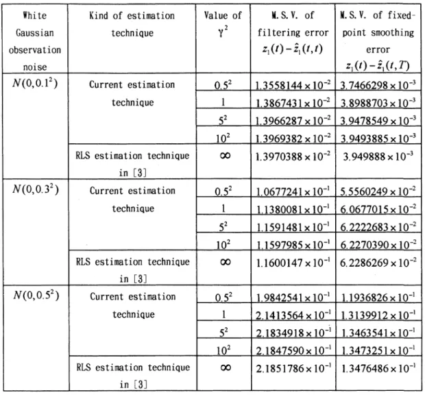
and the fixed-point smoothing estimate z¥ (t,T) when the observation noise obeys iV(0,0. 12), 7V(0,0.32) and Af(0,0.52).

White Kind of estima tion Value of M.S.V. of M.S.V. of fixedー

Gaussian technique Y 2 filtering error point smooth ing

observa tion noise *,(/) - *,(/,/) _error zA t) - zA t,T ) 〟 (0,0 .12) _{Current estimation} techn ique 0 .52 1.3 5 58 144 ×10 " 3.7 46 62 98 ×10 -3 1 1.3 86 74 3 1×10-2 _{3.89 88 70 3 ×io} -52 1.39 66 28 7 ×10 -2 3.9 47 854 9 ×10-3 102 1.39 69 3 82 ×10 -2 3.94 93 88 5 ×10-3 RLS estimation technique in 3 ∞ 1.39 70 3 88 ×10 -2 3.94 9 88 8 ×10 -3 A f(0,0 .32) _{Current estimation} technique 0.5^ 1.06 772 4 1×10" 5.5 560 24 9 ×10 -2 1 1.138 00 8 1 ×10-I 6 .06 7 70 15 ×10 -2 52 _{1.159 14 8 1 ×10"} 6 .22 2 26 83 ×10 -2 102 1.159 79 8 5 ×10 ' 6 .22 7 039 0 ×10 -2 RLS estimation techniaue in 3 ∞ 1.16 0 0 14 7 ×10 ーl 6.2 2 862 69 ×10 "

N (0,0 .52) _{Current estima tion}

techniQue

0 .52 1.984 2 54 1 ×10 " 1.19 36 82 6 x l0 -'

1 2 .14 13 56 4 ×10 " 1.3 13 99 12 ×10 "

52 _{2 .183 49 18 ×10 "} _{1.34 63 54 1 ×10 "}

10 2 2 .184 7 590 ×10 -1 1.34 73 25 1 ×i0 -1

RLS estima tion technique

in 3

∞ 2 .18 5 17 86 ×10 -I 1.34 764 8 6 ×10 "

the estimates for y =… in both cases of the filtering estimate z ¥{t,t) and the fixed-point smooth-ing estimate z i(t,T). The mean-square values are shown for the observation noises 7V(0,0. l2), 7V(0,0.32) and 7V(0,0.52). The mean-square values for the filtering and smoothing estimates of z¥(t) are calculated similarly with those of zi(i). For the filtering and fixed-point smoothing estimates, the mean-square values are evaluated for y2=0.52, 1, 52, 102. From Table 1 and Table 2, we find that the estimation accuracy of the smoothing estimates zi(t,T) and z ¥(t,T) is superior to the filtering estimates zi{tyi) and z ¥{t,i) respectively. Also, as the variance of the observation noise becomes small, the mean-square values of the filtering errors zi(i)-Z2(t,f) and z¥(t)-z i(t,t) and the smoothing errors z2(t)-zi(t,T) and z¥(t)-z ¥(t9T) become small. Clearly, the estimation accuracy of the estimates zi{tyi), z¥(t,t), zi(t,T) and zi(t,T) by the proposed

(29)

Design of Linear Stationary Stochastic Estimators in Relation to //<ォEstimation Technique 1 19

estimators is superior to that of the estimates for y2=- respectively. As the value of y2 in-creases, the mean-square values of the filtering errors z2(t)-z2{tyi) and z¥(t)-Z ¥(t,t) and the smoothing errors ziif)-Z2{t, T) and z¥(t)-z ¥(t,T) tend to be large.

8. Conclusions

The numerical simulation results have shown that the recursive suboptimal fixed-point

● ●

smoothing and filtering algorithms in [Theorem 4] are feasible. For y2=- the estimation algorithms for the fixed-point smoothing and filtering estimates in [Theorem 4] are same as

those by the RLS Wiener estimators [3] using the covariance information. For y2<-, the

estimation accuracy of the proposed estimators are preferable to those in [3].

In this paper, the stochastic estimation algorithms have been derived in a unified manner. By use of the covariance information, the optimal and suboptimal estimators have been

●

proposed respectively in [Theorem 3] and [Theorem 4] for linear continuous-time stochastic systems. The estimation algorithms for the fixed-point smoothing and filtering estimates of

● ●

z2(t)(=Lx(t)) and z¥(f)(-Cx(t)) have been obtained in relation to the deterministic 〃∞

estima-tion technique in the Krein spaces [1],[2].

In [Theorem 5] and [Theorem 6], by use of the state-space parameters, the optimal and suboptimal algorithms for the fixed-point smoothing and filtering estimates have been

de-● de-● de-●

rived respectively. The suboptimal filtering equations in [Theorem 6] using the state-space parameters are identical with those based on the game theory approach [5] in linear continu-ous systems. The suboptimal fixed-point smoother in [Theorem 6] is proposed for the first time in this paper.

References

[1] B. Hassibi, A. H. Saved andT. Kailath, "Linear Estimation in Krein Spaces - Part 1/ IEEE Trans. Automatic Control, Vol.41, no.l, pp.18-33, 1996.

[2] B. Hassibi, A. H. Sayed and T. Kailath, "Linear Estimation in Krein Spaces - Part II, IEEE Trans. Automatic Control, Vol.41, no. l, pp.34-49, 1996.

[3] S. Nakamori, Design of Recursive Wiener Smoother Given Covariance Information/ IEICE Trans. Fundamentals of Electronics, Communications and Computer Sciences, Vol.E79-A, pp.864-872, 1996.

[4] K.M. Nagpal and P.P Khargonekar, "Filtering and Smoothing in an //---Setting," IEEE Trans. Automatic Control, Vol.36, pp.151-166, 1991.

(30)

and Its Relation to the Minimum 〃∞-Norm Estimation, IEEE Trans. Automatic Control,

Vol.37, pp.828-831, 1992.

[6] I. Yaesh and U. Shaked, Game Theory Approach to Optimal Linear Estimation in

Mini-mum 〃∞-Norm Sense, Proceedings of the 28th Conference on Decision and Control, ■

pp.421-425, 1989.

[7] U. Shaked and Y. Theodor, "//｡｡-Optimal Estimation: A Tutorial, Proceedings IEEE Conference on Decision and Control, pp.2278-2286, 1992.

[8] I. Yaesh and U. Shaked, "Nondefinite Least Squares and its Relation to //｡｡-Minimum Error State Estimation, IEEE Trans. Automatic Control, Vol.36, no.12, pp.1469-1472,

1991.

[9] A.P. Sage and J.L. Melsa, Estimation Theory with Applications to Communications and Control, McGraw-Hill, 1971.

[10] L.M. Silverman, "Realization of Linear Dynamical Systems, IEEE Trans. Autom. Control, vol.AC-16, no.6, pp.554-567, Dec. 1971.