Inverse Problem for Electromagnetic Propagation in Human Muscle Tissues: Frequency Dependent Approach

全文

(1)Proceedings of the 51st ISCIE International Symposium on Stochastic Systems Theory and Its Applications Fukushima, Nov. 1-2, 2019. Inverse Problem for Electromagnetic Propagation in Human Muscle Tissues: Frequency Dependent Approach Fumio Kojima Professor Emeritus, Kobe University 1-1, Rokkodai-cho, Nada-ku, Kobe, 657-8501, Japan E-mail: [email protected] and H. T. Banks Center for Research in Scientific Computation North Carolina State University Raleigh, NC 27695-8212, USA E-mail: [email protected] Abstract This paper is concerned with an electromagnetic interrogation method for human muscle tissues using stochastic inversion methodology. The frequency dependence of relative permittivity of human muscle tissues is modeled by Debye formula with multiple dielectric relaxations. The associated signal response model is given by a complex reflectance at the interface between free space and the human body. The problem considered here is to identify posteriori distribution of the dielectric parameters from the measurements by a reflective interferometer. A computational experiments using Hamiltonian Monte Carlo sampling are summarized.. ing biological tissues. Dielectric relaxation measurements can analyze dielectric and electrical loss which provide useful and sensitive information on the human muscle tissues. Network analyzers are able to present a TDR view by transforming a frequency sweep to the time domain with a FFT.. 2. We consider a scattering problem for the region of interest ZROI = (0, z2 ) ⊂ R1 as illustrated in Fig. 1. A homogeneous dielectric material is assumed to be located at the interval (z1 , z2 ) ⊂ ZROI . Let Hy (t, z) be the magnetic field at the time t ∈ (0, t f ) at the location z ∈ ZROI .. 1 Introduction. x. Recently, electromagnetic imaging is of considerable interest in the signal detection and the identification related to the development of new ceramic materials, the early detection of anomalies in polymer, metabolic functioning of human bodies, etc [1]. Specifically, measurements for reflectance of microwave tests can be employed in the evaluation of the structural integrity of composite dielectric materials. This paper is focused on the identification and parameter estimation of human muscle tissues that entail treatments of individual parameters as random variables to be estimated from data. Our inversion technique is proposed based on classical Bayeasian approach using Markov Chain Monte Carlo sampling [2][3]. Previous efforts have been concentrated on problems of stochastic or statistical inverse problems that include some application to structural health monitoring [4] to [7]. In this paper, the method is effectively used for reconstructing a posteriori probability density functions of dielectric parameters for human muscle tissues. The ability to interrogate of tissues has wide ranging applications to medical imaging. Low amplitude and low energy microwaves can pass through dielectric media without caus-. – 28 –. Mathematical Model. Free Space. Dielectric Medium. Air Region. 0. Human Body. z1. z2 z. Interface. y. Fig. 1: Geometry of physical domain A planar electromagnetic wave Hy (t, z) normally incident on a dielectric material with faces parallel to the x − y plane. We also define the electric field E x (t, z) and the electric flux density D x (t, z) in (0, ∞) × ZROI . Those are polarized with oscillations in the x − z plane. Throughout the paper, we assume that the medium is composed of nonmagnetic material. Under these assumptions, Maxwell’s equations in ZROI.

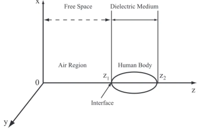
(2) can be represented by. Noting that. ∂Hy (t, z) ∂E x (t, z) = −µ0 ∂z ∂t in [0, ∞) × ZROI ∂Hy (t, z) ∂D x (t, z) = + σ0 E x (t, z) + Jyex (t, z) − ∂z ∂t in [0, ∞) × ZROI. bx (s, z) = P. k=1. (1). on ZROI. (3). In our formulation, the kernal function g is approximated by g(t) = ϵ0 (ϵ s − ϵ∞ ). m=1. (6). 0. (12). bx (ω, z) ∂E by (ω, z) = −ıµ0 ωH ∂z in (−∞, ∞) × (z1 , z2 ). (13). by (ω, z) ∂H bx (ω, z) − Jbyex (ω, z) = −ıϵ0 ωϵ ∗ (ω, z)E ∂z in (−∞, ∞) × (z1 , z2 ). (14). ∑ (ϵ s − ϵ∞ )gm σ0 + ıϵ0 ω m=1 1 + ıτm ω M. ϵr∗ (ω, z) B ϵ∞ +. for z1 < z < z2. bx B L[P x (t)], P Jbyex B L[Jyex (t)]. Then we obtain (8) (9). – 29 –. (15). The spectrum of dielectric media in human muscles involves multiple relaxation points. The feature of this model inM cludes the relaxation time {τm }i=1 and the weight coefficients M {gm }i=1 which means the contributions to the permittivity loss at each relaxation time. Let c = (µ0 ϵ0 )−0.5 be the speed of light and let {k = ω/(2πc)} be the interrogation wavenumber with respect √ to the specified angular frequency ωi . Setting as η0 = µ0 /ϵ0 , the complex permittivity is replaced by M η0 σ0 ∑ ∆ϵm ϵˆr (k) = ϵ∞ + + (16) 2πkı m=1 1 + ı(2πcτm )k where ∆ϵm = (ϵ s − ϵ∞ )gm .. where s = ψ + ıω. Similarly we define. bx (s, z) ∂E by (s, z) = −µ0 sH ∂z by (s, z) ∂H bx (s, z) − σ0 E bx (s, z) − Jbyex (s, z). = −sD ∂z. in C × (z1 , z2 ). In the frequency domain, the electromagnetic propagation in human muscle tissues can be obtained by substituting s = ıω into Eqs. (8) and (12). The frequency dependent model in a dielectric material can be expressed by. (5). Let us define the Laplace transform of the electrical field E x (t) by ∫ ∞ bx (s) B L[E x (t)] = E E(t, ·) exp(−st)dt (7). bx B L[D x (t)], D by B L[Hy (t)], H. − Jbyex (s, z). where ϵ ∗ is the complex relative permittivity defined by. where ϵ0 , ϵ s , and ϵ∞ denote the electric permittivity of free space, the static relative permittivity, and the permittivity at the very high frequencies of the medium, respectively. In Eq. (5), gk and τk imply the weight constant and the carrier relaxation time to be normally unknown. Allowing the instantaneous component of the polarization to be related to the electric field by a dielectric constant, the resulting constitutive law can be written by D x (t, z) = ϵ0 ϵ∞ E x (t, z) + P x (t, z).. (11). ( by (s, z) ∂H σ0 = −ϵ0 s ϵ∞ + ∂z ϵ0 s  M ∑ gm  b +(ϵ s − ϵ∞ )  E x (s, z) 1 + τm s  m=1. (2). 0. t exp(− ) τm τm. (10). Eq. (9) is rewritten by. where µ0 and σ0 denote the magnetic permeability of air and the electrical conductivity of the dielectric medium. To describe the behavior of the macroscopic electric polarization in the dielectric medium in human body, we assume that the polarization directly depend on the history of the electri∑K cal field. The dielectric polarization P(t, z) = k=1 Pk (t, z) can be then given by dielectric response function with a disK placement susceptibility kernel function {gk }k=1 (See [1] [8] for more details); ∫ ∞ P x (t, z) = g(t − ξ)E x (ξ, z)dξ. (4). M ∑ gm. gk b E x (s, z) 1 + τk s. bx (s, z) = ϵ0 ϵ∞ E bx (s, z) + P bx (s, z), D. with the initial state E x (0, z) = Hy (0, z) = 0. K ∑. (17). The purpose of this study is to identify the unknown parameM ters {τm , ∆ϵm }m=1 through the measurements by electromagnetic microscopy. The reflective coefficient r at the plane interface between air and a dielectric medium is given by √ 1 − ϵˆr (k) (18) r(k) = √ 1 + ϵˆr (k) Then, by sweeping frequencies over ten decades, measurements provide the observable reflectance [9] given by R(ki ) = r(ki )r(ki ),. ki = fi /c for i = 0, 1, · · · , N−1. (19).

(3) Observation data can be performed in time domain and the collected data are transformed into the spectrum using the DFT.. 3. with the equality constraint: qm+M η0 σ0 ∑ + . 2πkı m=1 1 + ı(2πcqm )k M. ϵˆr (k, q M ) = ϵ∞ +. (27). Formulation of the Problem. Let Q M be a random vector on the probability triple (Ω, F , P). Assuming that random variables Qi are mutually independent, the joint distribution of Q M is represented by FQM (q M ) =. M ∏. =. P(Qm ≤ qm ). for q M ∈ R M .. (20). m=1. The associated joint prior density functions for Q M can be represented by πQM (q M ) =. M ∏. πm (qm ). (21). m=1. where πm (qm ) =. dF Qm (qm ) dqm. for i = 1, 2, · · · , M.. (22). Our inverse problem treated here is to identify the unknown M parameter vector q M = {τm , ∆ϵm }m=1 ∈ R2M based on the N−1 observable reflectance {R(ki )}i=0 . Hence the prior density of unknown parameters q M can be represented by the product form: πQM (q M ) =. M ∏. πm (qm ). m=1. = π(τ1 ) × π(τ2 ) × · · · × π(τm ) × π(∆ϵ1 ) × π(∆ϵ2 ) × · · · × π(∆ϵm ). (23). N−1 It is a natural way that the real data Yd = {yd (ki )}i=0 are corrupted with measurement noise. Hence we assume that the residual term. has the statistical distribution: ( ) ηi ∼ πe yd (ki ) − R(ki , q M ) for i = 0, 1, · · · , N − 1. (24) N−1 {ηi }i=0. Suppose that sequence of measurement errors are mutually independent measurement. Then the likelihood ratio function can be represented by N−1 ∏. πe (yi − R(ki , q M )).. (25). An estimation algorithm can be performed by sampling procedures for the posteriori distribution density π(q M ) from which sample paths can be drawn using Markov chains. There are many alternative algorithms of MCMC, such as Metropolis-Hasting (MH), Gibbs sampling methods, etc (See, [3]). Our prior efforts on material characterizations exist using independent Metropolis-Hastings [4], gPC Galerkin method [5], and the stochastic spline Galerkin method [6]. Those have been performed using time domain approach (the so-called “snapshot method”). The crucial aspects on our previous efforts involved spending the heavy computational times for practical implementation of the sampling procedures. As a result, the asymptotic behavior of the sampling process is not especially well suited for identifying multi-dimensional unknown quantities. Recently, an estimation scheme using Hamiltonian Monte Carlo method (HMC) was applied to the inverse problem for Dobye model for composite materials [7]. The method is a Metropolis method making use of gradient information to reduce random walk behavior. HMC has the advantages on the asymptotic behavior of MCMC sampling [10]. In HMC,the state space z = q M is augmented by momentum variables p. Let us define the Hamiltonian H(z, p) = E(z) + K(p). (29). where K is a kinetic energy. Then the algorithm is used to create samples from the joint density 1 exp {−H(z, p)} CH 1 = exp {−E(z)} exp {−K(p)} . CH. Thus our inverse problem is stated as follows: (IP): Given a prior distribution πQM (q M ) and the collection N−1 of the measurement data {yd (ki )}i=0 , estimate posterior denM sity π(q ) of unknown quantities (26). – 30 –. (30). The continuous form of the sampling mechanism can be described by the differential rule { z˙ = p . (31) p˙ = −∂E(z)/∂z The the explicit form of E in our inversion is described by E(z) = log C + log πe (Yd − Y(z)) + log πZ (z). i=0. M M q M = {qm , qm+M }m=1 = {τm , ∆ϵm }m=1. (28). πˆ H (z, p) =. ηi = yd (ki ) − R(ki , q M ). L(y0 , y1 , · · · , yN−1 |q M ) =. From the Bayes formula, the posterior probability density function has the representation π(q M ) ∝ L(y0 , y1 , · · · , yN−1 |q M )πQM (q M ).. F Qm (qm ). m=1 M ∏. 4 Inverse Methodology. (32). where C denotes the normalizing factor and where N−1 . Y(z) = {R(ki , z)}i=0. (33). In this paper, the same scheme is adopted to the problem for human muscle tissues..

(4) 5. Computational Experiments. 5.1 Forward Analysis Gabriel et al.[11][12] carried out an experimental study on a large number of biological tissues spanning the frequency range from 10Hz to 20GHz. Figure 2 depicts the model reflectance for N = 100 using the parameter values in Table 1for the case of M = 1, 2, 3, 4, 5. Throughout the experiments, we set as ϵ∞ = 4.3, σ0 = 0.0762.. σe ∼ InvGamma(α, β), ( L U) f m , f m , (m = 1, 2, · · · , 5) τ−1 ∼ Uniform m ( L ) U (m = 1, 2, · · · , 5) ∆ϵm ∼ Uniform ∆ϵ m , ∆ϵ m. for i = 0, 1, 2, · · · N.. In the experiments, we set as fL = 10, fH = 5.0 × 1010 , and N = 10000.. σe = 0.01,. α = 1.0,. (37). β = 1.0.. ∆ϵm 8 × 105 81900 11900 32 46. 6000. density.default(x = tau1). 4000 3000 0. 1000. 2000. Density. 5000. τ−1 m 69[Hz] 43[kHz] 670[kHz] 230[MHz] 20[GHz]. (36). In the experiments, the HMC sampling using R-stan language code was adopted to our inversion [13]. Figures 5 to 12 show the marginal posteriori density plots for the unknown parameters. Tables 2 to 3 summarize the estimated values of the unknown quantities.. Table 1: Relaxation parameters for human muscle tissue m 1 2 3 4 5. (35). where all the statistical parameters of a prior distributions are given. Syntheses data were used by computing the forward problem provided with true parameters and by adding the Gaussian random noise to those data. Those were preassigned as. The wavenumber was taken as ki = 10{log( fL )+log( fH / fL )(i/N)}. 5.2 Inverse Analysis The nonlinear hierarchical models used in the inversion technique are formulated as: ( ) yi ∼ Normal R(ki ; q M ), σe (34). 0.0115. 0.0120. 0.0125. N = 100000 Bandwidth = 9.384e−06. Fig. 3: Recovered posterior density π(τ1 ). 0.0e+00. Density. Fig. 2: The simulated reflectance in human muscle model for the case M = 1, 2, 3, 4, 5. 1.0e+08. 2.0e+08. density.default(x = tau2). 2.000e−05. 2.001e−05. 2.002e−05. 2.003e−05. 2.004e−05. N = 100000 Bandwidth = 2.446e−10. Fig. 4: Recovered posterior density π(τ2 ). – 31 –.

(5) density.default(x = deps2). 0.03 0.02. Density. 4e+09. 0.00. 0e+00. 0.01. 2e+09. Density. 0.04. 6e+09. 0.05. density.default(x = tau3). 1.4285e−06. 1.4290e−06. 1.4295e−06. 1.4300e−06. 89850. 89900. N = 100000 Bandwidth = 8.755e−12. 89950. 90000. N = 100000 Bandwidth = 1.116. Fig. 5: Recovered posterior density π(τ3 ). Fig. 9: Recovered posterior density π(∆ϵ2 ). density.default(x = deps3). 0.6 0.4. Density. 0.0. 0.0e+00. 0.2. 1.0e+10. Density. 2.0e+10. 0.8. density.default(x = tau4). 3.35e−09. 3.40e−09. 3.45e−09. 3.50e−09. 3.55e−09. 3.60e−09. 3.65e−09. 12988. 12990. 12992. N = 100000 Bandwidth = 2.363e−12. 12994. 12996. 12998. 13000. N = 100000 Bandwidth = 0.07783. Fig. 6: Recovered posterior density π(τ4 ). Fig. 10: Recovered posterior density π(∆ϵ3 ). density.default(x = deps4). 25 20. Density. 0. 0e+00. 5. 10. 15. 4e+11 2e+11. Density. 6e+11. 30. 35. 8e+11. density.default(x = tau5). 5.3e−11. 5.4e−11. 5.5e−11. 5.6e−11. 5.7e−11. 49.75. 49.80. N = 100000 Bandwidth = 4.298e−14. Fig. 7: Recovered posterior density π(τ5 ). 49.90. 49.95. 50.00. Fig. 11: Recovered posterior density π(∆ϵ4 ). density.default(x = deps5). 10 0. 0e+00. 5. 2e−05. Density. 4e−05. 15. 6e−05. density.default(x = deps1). Density. 49.85. N = 100000 Bandwidth = 0.001712. 780000. 800000. 820000. 840000. 860000. 880000. 900000. 49.5. N = 100000 Bandwidth = 877.8. 49.6. 49.7. 49.8. 49.9. 50.0. N = 100000 Bandwidth = 0.003445. Fig. 8: Recovered posterior density π(∆ϵ1 ). Fig. 12: Recovered posterior density π(∆ϵ5 ). – 32 –.

(6) [3] D. Gamerman: Markov Chain Monte Carlo, Stochastic Simulation for Bayesian Inference, Chapman & Hall, New York, 1997.. Table 2: Test Summary (τm ) m. True. Mean. 1 2 3 4 5. 1.45 × 10−2 2.33 × 10−5 1.49 × 10−6 4.35 × 10−9 5.00 × 10−11. 1.12 × 10−2 2.00 × 10−5 1.43 × 10−6 3.37 × 10−9 5.49 × 10−11. Standard Deviation 1.30 × 10−4 3.28 × 10−9 1.18 × 10−10 2.99 × 10−11 4.79 × 10−13. [4] F. Kojima and J.S. Knopp; Inverse problem for electromagnetic propagation in a dielectric medium using Markov Chain Monte Carlo method, International Journal of Innovative Computing, Information and Control (IJICIC), 8, pp.2339-2346, 2012. [5] F. Kojima, Y. Fujiwara, and T. Usami: Inverse analysis for dielectric medium of conducting materials using generalized polynomial Chaos Galerkin method, Proc. SICE Annual Conference 2014, Sapporo, Japan, 2014.. Table 3: Test Summary (∆ϵm ) m. True. Mean. 1 2 3 4 5. 8.00 × 10 8.19 × 104 1.19 × 104 3.20 × 10 4.60 × 10 5. 8.88 × 10 9.00 × 104 1.30 × 104 5.00 × 10 5.00 × 10 5. Standard Deviation 1.13 × 104 1.50 × 10 1.06 2.31 × 10−2 4.63 × 10−2. [6] F. Kojima and T. Usami: Estimation of dielectric parameters in composite materials using stochastic Galerkin method, Proc. SICE Annual Conference 2015, Hangzhou, China,2015. [7] F. Kojima and H.T. Banks: Statistical parameter estimation of dielectric materials using MCMC for nonlinear hierarchical models, International Journal of Applied Electromagnetics and Mechanics, 52-2, pp.4954,2016.. 6 Concluding Remarks Stochastic inverse methodologies for dielectric components of composite materials were investigated. The physical model given by the Debye model was considered for identifying the time relaxation parameters in human muscle tissues. Nonlinear hierarchical regression models were constructed in order to implement MCMC sampling. The feasibility studies were demonstrated by computational experiments using the simulated data analysis. Feasibility studies were carried out illustrating the method with computational experiments using the same simulated data. The consistency of estimated values can be demonstrated by the estimated marginal densities from extracting sampling results which were able to provide the reliability and uncertainty quantification for the associated inverse solutions.. Acknowledgements Part of this research was carried out while the first author was visiting at Center for Research in Scientific Computation (CRSC), North Carolina State University.. [8] C. J. F. Bottcher and P. Bordewijk: Theory of Electric Polarization, Second Edition, Elsevier, Amsterdam, 1978. [9] H.T. Banks, J. Catenacci and S. Hu: Estimation of distributed parameters in permittivity models of composite dielectric materials using reflectance, J. Inverse and Ill-posed Problems, 23-5 pp.491-509 2015. [10] R.M. Neal: MCMC using Hamiltonian Dynamics, Handbook of Markov Chain Monte Carlo, Eds. S. Brooks, A. Gelman, G. Jones, and X. Meng, Chapman & Hall, CRC Press, London, 2011. [11] C. Gabriel, S. Gabriel, and E. Corthout: The dielectric properties of biological tissues: I. Literature survey, Phys. Med. Biol. 41, pp.2231-2249, 1996. [12] S. Gabriel, R.W. Lau, and C. Gabriel: The dielectric properties of biological tissues: II. Measurements in the frequency range of 10Hz to 20GHz, Phys. Med. Biol. 41, pp.2251-2269, 1996. [13] Stan Development Team: Stan Modeling Language Users Guide and Reference Manual, Ver. 2.6.0, http://mc-stan.org/ February 2015.. References [1] H. T. Banks, M.W. Buksas and T. Lin: Electromagnetic Material Interrogation Using Conductive Interfaces and Acoustic Wavefronts, Frontier in Applied Mathematics, FR21, SIAM, Philadelphia, 2000. [2] W. R. Gilks, S. Richardson and D. J. Spiegelhaltger: Markov Chain Monte Carlo in Practice, Chapman & Hall/CRC, New York, 1996.. – 33 –.

(7)