福岡工業大学学術機関リポジトリ

(1)

using Dynamic Programming Approach

By

BD17103

Rachanart Soontornvorn

Supervisor

Prof. Dr. Hiroyuki Fujioka

A thesis submitted in partial fulfilment

of the requirements for the degree of

Doctor of Engineering

Intelligent Information System Engineering

Fukuoka Institute of Technology

Fukuoka, Japan

c

(2)

(3)

I would never have been able to finish my dissertation without the guidance of my advisor, help from friends, and support from my family.

Firstly, I would like to express my gratitude to my supervisor Professor Hiroyuki Fujioka of the Department of System Management Engineering at Fukuoka Institute of Technology. His expertise, understanding, and patience, added considerably to my graduate experience. I appreciate his vast knowledge and skill in many areas and for his continuous support of my doctor’s degree study and related research. He provided me with an excellent atmosphere for doing research. His guidance helped me all the time with researching and writing this thesis. For six years from my master’s degree until my doctor’s degree, he always advised me not only with academic problems, but also whenever I had terrible situation. He always pushed me to be better. I am so proud to be the part of Fujioka Laboratory as his student.

I would like to thank Professor Takuya Tajima, Professor Yu Song from the Department of System Management Engineering and Professor Hitoshi Kino from the Department of Intelligent Mechanical Engineering for giving valuable advices to write this thesis. Also, I would like to thank Assistant Professor Vanvisa Chutchavong from Department of Computer Engineering, Faculty of Engineering at King Mongkut’s Institute of Technology Ladkrabang Bangkok, Thailand, and Associate Profes-sor Kanok Janchitrapongvej, Faculty of Science and Technology Southeast Bangkok College (SBC), Bangkok, Thailand, for giving me precious opportunities to discuss on this work. I would like to thank every member of Fujioka Laboratory. They always helped me and give me advices many times. My research would not have been possible without their help. Moreover, I would like to thank all of the staff of International Affairs at Fukuoka Institute of Technology. In particular, Ms. Fumie Yuki who teach Japanese language and always supported me in all of my Japanese life. Without her support, I could not have accomplished this thesis.

Finally, I would like to thank my family, Mr. Chupong Soontornvorn, Mrs. Krongkaeo Soontornvorn and Ms. Chayada Ukarawongchai for supporting me spiritually throughout writing this thesis and my life in general.

Rachanart Soontornvorn Intelligent Information System Engineering BD17103

(4)

(5)

Fitting a curve to a set of data points is a key problem in many applications of science and engineering such as numerical analysis, robotics and image processing, etc. For solving such a curve-fitting problem, a natural approach is one with the so-called “spline function” which is a special function defined by piecewise polynomials. Such a spline approach enables us to yield the simplicity of their construction, their ease and accuracy of evaluation, and their capacity to approximate complex shapes through curve-fitting and interactive curve design. In particular, a natural choice from various types of splines is ‘B-splines’ developed by Schoenberg, in which a spline function has minimal support with respect to a given degree, smoothness, and domain partition.

This thesis considers a problem of designing curves using B-spline approach. Therein, the curves are constituted by employing the normalized, uniform B-splines as basis functions. That is, their knot points are equally-spaced. Then, a sequence of control points of B-splines is called as ‘control polygon’, which represents the geometrical outline of curves. Such a treatment on the control polygon is very powerful in the interactive curve design. With respect to the design using such a B-spline approach, we however see that the design usability may depend on the number of control points on the curves. For improving such a design usability, a natural way is to represent some given planar curves as more compact B-spline curves by using only the dominant control points, in which the desired approximation accuracy is achieved.

Main purpose of thesis is to develop a method for designing such compact B-spline curves by using only the dominant control points. In particular, such a method is developed for typical two types of B-spline curves, i.e., “planar B-spline curves” and “periodic B-spline curves”. Then, a central issue is how we optimally select a dominant control points. For solving such a problem, we here introduce an optimization approach using dynamic programming (DP) method. That is, the selection problem is formulated as a graph problem and is solved by dynamic programming. Thus, the method does not lead to huge amounts of computation time unlike the ordinary approaches - such as trial-and-error approach, etc. In addition, it is shown that representation using the selected control points can be realized using NURBS (Non-Uniform Rational B-splines). The proposed methods for the planar and periodic splines can be applied to the character design using the so-called dynamic font method and the contour modeling problem for the deformable objects, respectively. The performances are demonstrated by experimental studies.

(6)

(7)

Acknowledgements

Abstract

1 Introduction 1

2 Spline Curve Basics 5

2.1 Introduction . . . 5

2.2 Power Basis Form of a Curves . . . 5

2.3 B´ezier Curves . . . 6

2.3.1 Rational B´ezier Curves . . . 10

2.4 B-spline Curves . . . 11

2.4.1 B-spline Basis Functions . . . 12

2.4.2 B-spline Curves . . . 15

2.5 NURBS . . . 18

3 Dynamic Programming Approach 22 3.1 Introduction . . . 22

3.2 Graph . . . 22 i

(8)

3.2.2 Directed Graph . . . 23

3.2.3 Directed Acyclic Graph . . . 25

3.3 Dynamic Programming . . . 26

3.3.1 Dynamic Programming Algorithms . . . 27

4 A Design of Compact Planar B-spline Curves 28 4.1 Introduction . . . 28

4.2 Problem Statement . . . 29

4.3 Reconstructing Compact Planar B-spline Curves using DP Control Point Selection . 31 4.3.1 Optimal Control Point Selection using Dynamic Programming for Compact Planar B-spline Curves . . . 31

4.3.2 Representing Compact Planar B-spline Curves using Non-Uniform Rational B-splines (NURBS) . . . 33

4.4 Experimental Study . . . 36

5 A Design of Compact Periodic B-splines Curves 60 5.1 Introduction . . . 60

5.2 Periodic B-spline Curves . . . 61

5.3 Reconstructing Compact Periodic B-spline Curves using DP Control Point Selection 62 5.3.1 Optimal Control Point Selection using Dynamic Programming for Compact Periodic B-spline Curves . . . 62

5.3.2 Representing Compact Periodic B-spline Curves using Non-Uniform Ratio-nal B-splines (NURBS) . . . 63

5.4 Experimental Study . . . 64 ii

(9)

Bibliography 78

Publications 84

(10)

2.1 Quadratic B´ezier Curves. . . 7

2.2 Cubic B´ezier Curves. . . 7

2.3 The basis function Bi,n(t) for n = 3, 5, and 9. . . 9

2.4 Design examples of B´ezier curves and Rational B´ezier curves. . . 12

2.5 An example of B-spline basis functions. . . 14

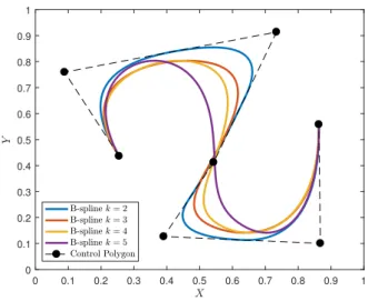
2.6 B-spline curves of degree k = 2, 3, 4 and 5 with the control polygons. . . 17

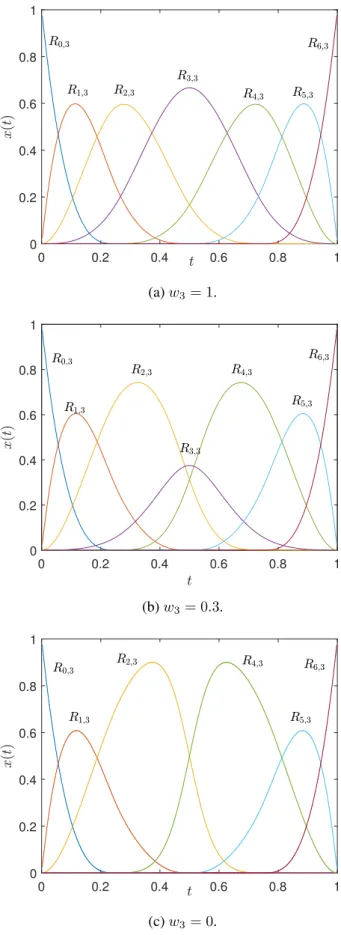
2.7 Rational cubic B-spline curves with w3 varying. . . 20

2.8 The cubic basis functions for the curves in Figure 2.7 with w3varying. . . 21

3.1 An example of a simple graph. . . 23

3.2 An example directed graph or digraph. . . 25

3.3 An example of directed acyclic graph (DAG). . . 26

4.1 Given planar data curves represented on O − XY plane and its control polygon M with a set of handwriting. . . 39

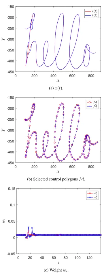
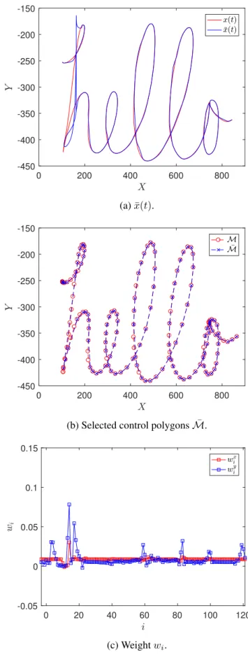
4.2 Compact planar B-spline curves for the case of “hello” with lmax = 0, K = 139 ( ¯M = 143). . . 40

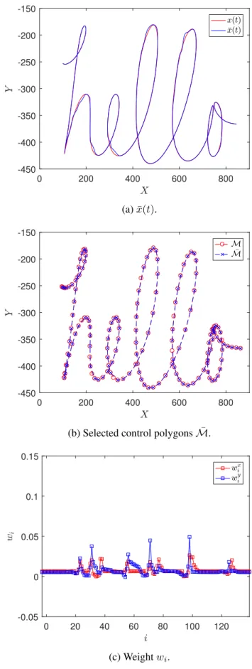
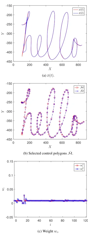
4.3 Compact planar B-spline curves for the case of “hello” with lmax = 1, K = 139 ( ¯M = 143). . . 41

(11)

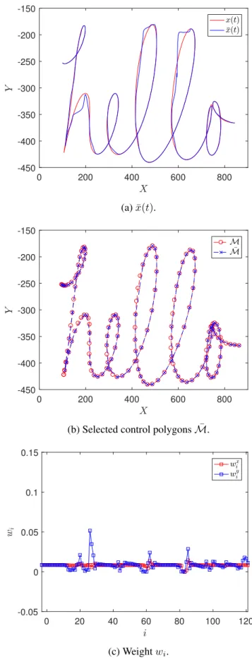
4.5 Compact planar B-spline curves for the case of “hello” with lmax = 0, K = 121

( ¯M = 125). . . 43 4.6 Compact planar B-spline curves for the case of “hello” with lmax = 1, K = 121

( ¯M = 125). . . 44 4.7 Compact planar B-spline curves for the case of “hello” with lmax = 2, K = 121

( ¯M = 125). . . 45 4.8 Compact planar B-spline curves for the case of “fukuoka” with lmax = 0, K = 197

( ¯M = 175) . . . 49 4.12 Compact planar B-spline curves for the case of “fukuoka” with lmax = 1, K = 171

( ¯M = 175). . . 51 4.14 Compact planar B-spline curves for the case of “welcome” with lmax = 0, K = 130

( ¯M = 134). . . 54 v

(12)

4.18 Compact planar B-spline curves for the case of “welcome” with lmax = 1, K = 113

( ¯M = 117). . . 57 4.20 RMSE for all the case of K, lmax = 0, 1 and 2. . . 58

4.21 Compact planar B-spline curves ¯x(t) for the cases of “hello”, “fukuoka”, and “wel-come”, where the control points are randomly selected. . . 59

5.1 Designed periodic B-spline curve x(t). . . 65 5.2 Result of Compact periodic B-spline curves when lmax = 0, K = 31 ( ¯M = 35). . . . 67

5.3 Result of Compact periodic B-spline curves when lmax = 1, K = 31 ( ¯M = 35). . . . 68

5.11 Compact periodic B-spline curves ¯x(t) for the case where the control points are ran-domly selected. . . 75

(13)

4.1 The total number of control points M and the time interval [t0, tm] for the cases of

“hello”, “fukuoka” and “welcome”. . . 38 4.2 Setup on the number of selected control points K ( ¯M ) for the results of “hello”,

“fukuoka” and “welcome” in a result for Figures 4.2-4.19. . . 38

(14)

(15)

Introduction

Curve-fitting is the problem of constructing a curve (i.e., some mathematical function) that has the best fit to a series of data points, possibly subject to constraints. Such a curve fitting involves either interpolation or smoothing. Here, the former indicates that an exact fit to the data is required, On the other hand, the later indicates that a “smooth” function is constructed that approximately fits the data. The curve-fitting problem to a given set of data may arise in many applications of science and engineering such as statistics [1], [2], numerical analysis [3]-[5], image processing [6]-[8], robotics [9]-[12], etc., For example, in [13], the motion planning problem for mechanical systems has been treated as the curve-fitting problem. For solving such a curve-fitting problem, a natural approach is one with the so-called “spline function” which is a special function defined by piecewise polynomials. Such a spline approach enables us to yield the simplicity of their construction, their ease, and accuracy of evaluation, and their capacity to approximate complex shapes through curve fitting and interactive curve design. In particular, a natural choice from various types of splines is ‘B-splines’ developed by Schoenberg [14], and [15], in which a spline function has minimal support with respect to a given degree, smoothness, and domain partition. Fujioka and Kano have also studied the optimal design and properties of curves and surfaces by using the B-spline approach (e.g., [16]). Therein, they have analyzed the convergence properties of interpolating and smoothing splines as the number of data increases to the infinity [17]. Also, various types of splines - such as planar splines, periodic splines, and constrained splines, etc. have been developed. In this thesis, we restrict ourselves to the problem on the planar spline curves and periodic spline curves.

The planar spline curves are curves that can be represented in Cartesian coordinates by a parametric 1

(16)

equation of the form (x, y) = (x(t), y(t)) for spline curves x(t) and y(t) [18] and [19]. For example, Bo’s work in [20] has exhibited the fundamental planar curve-fitting problem to unorganized data points by introducing B-splines. As for its applications, the planar spline curves have been applied to the geometric modeling problem. Another typical example is described in Morgand’s work [21], in which planar spline curves are used to predict the shape of specularities by introducing some planar B-splines. Similar work has been exhibited in Kim’s work [22]. Therein, the planar spline curves have been used to plan the robotic motion in the geometric environment using some algebraic algorithms. Also, there is another application which we are very interested. The application is a design of character font based on the so-called “dynamic font” developed by Takayama and Kano in [23]. The dynamic font method has been developed by mimicking the writing process by humans, in which characters are generated by moving a writing device on a writing plane continuously in both time and space. This method is powerful, particularly when we want to generate and manipulate characters in Japanese calligraphy where the thickness of the stroke is important. Such a motion is generated by using normalized uniform B-spline as a basis function. The sequence of control points of B-splines is called as ‘control polygon’, which represents the geometrical outline of curves. Such a property leads many advantages to manipulate characters. For example, the operations on characters - such as resize, translation, rotation, and concatenation, etc. can be defined as operations on control polygon [24].

On the other hand, the periodic spline curves are curves that repeat its values in regular intervals or periods using splines [25]. A typical mathematical example of using such periodic spline curves may be to interpolate or approximate the trigonometric functions, which repeat over intervals of 2π radians. In addition, such periodic spline curves may be used throughout science to describe oscillations, waves, and other phenomena that exhibit periodicity [26]. Also, Fujioka and Kano’s group has studied the optimal design of such periodic spline curves by using B-spline approach and control-theoretic approach and their result has been applied to the contour modeling of wet material objects - such as jellyfish and red blood cell, etc. [17]. Similar works on periodic spline curves have been appeared in the field of computer vision such as the idea of matching systems for contour the human face and head based on periodic curvature in [27].

This thesis considers the problem of designing curves using the B-spline approach. Therein, the curves are constituted by employing the normalized, uniform B-splines as basis functions. That is, their knot points are equally-spaced. Then, a sequence of control points of B-splines is called as

(17)

‘control polygon’, which represents the geometrical outline of curves. Such a treatment on the control polygon is very powerful in the curve design problem. As mentioned above, in the case of dynamic font using planar spline curves, manipulations on characters can be defined as some operations on the control polygon. Also, in the case of contour modeling using periodic spline curves, such a treatment yield an efficient algorithm to understand the deformation motion, etc. More specifically, the computation on the area and shape complexity can be given by simple functions in terms of control point vector (i.e., control polygon). With respect to the design using such a B-spline approach, we, however, see that the design usability depends on the number of control points on the curves. For improving such design usability and computation speed in the algorithm, a natural way is to represent a given spline-curves as more compact B-spline curves by using only the dominant control points, in which the desired approximation accuracy is achieved.

The main purpose of this thesis is to develop a method for designing such compact B-spline curves by using only the dominant control points. In particular, such a method is developed for typical two types of B-spline curves i.e., “planar B-spline curves” and “periodic B-spline curves”. Then, a cen-tral issue is how we optimally select dominant control points. For such an optimal dominant control point selection, the most typical approach may be the trial-and-error approach exhibited in Lyche and Mørkens work [28]. Therein, a larger number of control points is initially defined, and then, certain knot points are greedily removed by employing some heuristic criterion. After removing the knot points, recomputing the control points is required in order to achieve the desired approxima-tion accuracy. Similar work is exhibited in Park and Lee’s work [29]. However, it is well-known that the trial-and-error approaches lead to huge amounts of computation time. On the other hand, Tjahjowidodo et al. [30] have recently developed a fast algorithm for optimally finding knot points using the so-called half-split method, where it is limited to the case of cubic splines. The basic idea is to approximate a subset of the second derivative sample points as a set of piecewise linear functions. This may be applicable to cases where we want to select dominant control points from original ones. But, it may be impossible to apply this method when we want to specify the number of dominant control points, as in the following discussion of this study.

For solving such a selection problem, we here introduce an optimization approach using a dynamic programming (DP) method. That is, the selection problem is formulated as a graph problem and is solved by dynamic programming. Thus, the method does not lead to huge amounts of computation time unlike the ordinary approaches - such as the trial-and-error approach [30]. Then, we have only

(18)

to represent our compact B-spline curves. Since the intervals between their knot points may be non-uniform, representing dominant control point to our compact B-spline curves is achieved by using Non-Uniform Rational B-Splines (NURBS). The methods for the planar and periodic splines can be applied to the character design using the so-called dynamic font method [23] and the contour modeling problem for the deformable objects [31], respectively. The performances are demonstrated by experimental studies.

The outline of this thesis is as follows. In Chapter 1, we give the background and the purpose of this thesis as an introduction. In Chapter 2, we present the spline curve basics including B-spline as well as Non-Uniform B-splines (NURBS), which will be frequently used throughout this thesis. In Chapter 3, we present the dynamic programming including a graph theory. In Chapter 4, we develop the method for designing compact planer B-spline curves and conduct some experimental studies in order to demonstrate the usefulness and effectiveness of our proposed method. The similar work for the case of periodic splines are discussed in Chapter 5. In Chapter 6, concluding remarks of this thesis are given.

(19)

Spline Curve Basics

2.1 Introduction

In this chapter, we present the spline curve basics. In Section 2.2, we present the power basis form of a curve, which is a common method for expressing polynomial functions. Then, the B´ezier curves are introduced in Section 2.3. In Section 2.4 and 2.5, we present the B-spline curves and NURBS (Non-Uniform Rational B-spline), which will be used throughout in this thesis.

2.2 Power Basis Form of a Curves

We first present the power basis form for a curves, which is a common method for expressing poly-nomial functions.

Let x(t) be n-th degree power basis curves, then we have

x(t) =

n

X

i=0

aiti. (2.1)

Also, this can be written in matrix form as

(20)

x(t) = [a0 a1 · · · an]         1 t .. . ti         = [ai]T[ui]. (2.2)

Differentiating (2.1) in terms of t may give as

ai =

xi(t)|t=0

i! , (2.3)

where xi(t)|t=0is the i-th derivative of x(t) at t = 0. We here call the n + 1 function t’s as the basis

functions. Also, ai’s are called as coefficients of the power basis presentation.

It can be shown that the point x(t) on power basis curves can be computed efficiently by introducing Horner’s method as follows,

for n = 1, x(t0) = a1t0 + a0 n = 2, x(t0) = (a2t0+ a1)t0+ a0 .. . n = ¯n, x(t0) = ((· · · (¯ant0+ ¯an−1)t0+ ¯an−2)t0+ · · · + a0 . (2.4)

2.3 B´ezier Curves

We next present Bézier curves, which are parametric polynomial curves. Since the power basis form uses polynomials for the representation of curves, thus the Bézier form is mathematically equivalent to the power basis form. That is, any curves that can be represented in the Bézier form can be represented in the power basis forms. However, the Bézier curves have been frequently used in some software - such as the modeling and drawing tools due to the drawbacks of the power basis forms (i.e., huge computational cost, etc.).

(21)

x(t) =

n

X

i=0

piBi,n(t) 0 ≤ t ≤ 1, (2.5)

where Bi,n(·) denotes the n-th degree Bernstein polynomials given by

Bi,n(t) =

n! i!(n − i)!t

i_{(1 − t)}n−i _{t ∈ [0, 1].} _(2.6)

The coefficients pi are called “control points” that approximate the shape of the curve. Figures 2.1

and 2.2 illustrate design examples of quadratic and cubic B´ezier curves, where we note that x(t) is defined as x(t) = [X(t) Y (t)]T ∈ R2. 0 1 2 3 4 5 6 7 8 0 0.5 1 1.5 2 2.5 3 3.5 4 4.5 5 5.5

Figure 2.1: Quadratic B´ezier Curves.

0 1 2 3 4 5 6 7 8 0 0.5 1 1.5 2 2.5 3 3.5 4 4.5 5 5.5

(22)

The B´ezier curves are invariant under the usual transformations such as rotations and translations, and others by applies the transformation it to the control polygon. Normally, the choice of basis function determines the geometric characteristic of the scheme. The properties of basis function Bi,n(t) degree

n (i.e., degree n = 3, 5 and 9 in Figures 2.3) can be summarized as follows,

• Non-negativity : Bi,n(t) ≥ 0, 0 ≤ t ≤ 1.

• Partition of unity : Pn

i=0Bi,n(t) = 1, 0 ≤ t ≤ 1.

• B0,n(0) = Bn,n(1) = 1.

• Bi,n(t) attains exactly one maximum on the interval [0,1], that is, at t = _ni.

• Symmetry : for any n, the set of polynomial Bi,n(t) is symmetric with respect to t = 1₂.

• Recursive definition : Bi,n(t) = (1 − t)Bi,n−1(t) + tBi−1,n−1(t); we define Bi,n(t) ≡ 0, if i <

0 or i > n. • Derivative : B0

i,n(t) =

dBi,n(t)

dt = n(Bi−1,n−1(t) − Bi,n−1(t)) with B−1,n−1(t) ≡ Bn,n−1(t) ≡ 0.

For example, we can calculate Bi,n(t) for the cubic case (i.e., n = 3) as

B0,1(t) = (1 − t)B0,0(t) + tB−1,0(t) = 1 − t B1,1(t) = (1 − t)B1,0(t) + tB0,0(t) = t B0,2(t) = (1 − t)B0,1(t) + tB−1,1(t) = (1 − t)2 B1,2(t) = (1 − t)B1,1(t) + tB0,1(t) = 2t(1 − t) B2,2(t) = (1 − t)B2,1(t) + tB1,1(t) = t2 B0,3(t) = (1 − t)B0,2(t) + tB−1,2(t) = (1 − t)3 B1,3(t) = (1 − t)B1,2(t) + tB0,2(t) = 3t(1 − t)2 B2,3(t) = (1 − t)B2,2(t) + tB1,2(t)3t2(1 − t) B3,3(t) = (1 − t)B3,2(t) + tB2,2(t)t3 . (2.7)

Using the property of recursive definition and derivative, the general expression on the derivative of a B´ezier curves can be obtained as

(23)

0 0.1 0.2 0.3 0.4 0.5 0.6 0.7 0.8 0.9 1 0 0.1 0.2 0.3 0.4 0.5 0.6 0.7 0.8 0.9 1 (a) n = 3. 0 0.1 0.2 0.3 0.4 0.5 0.6 0.7 0.8 0.9 1 0 0.1 0.2 0.3 0.4 0.5 0.6 0.7 0.8 0.9 1 (b) n = 5. 0 0.1 0.2 0.3 0.4 0.5 0.6 0.7 0.8 0.9 1 0 0.1 0.2 0.3 0.4 0.5 0.6 0.7 0.8 0.9 1 (c) n = 9.

(24)

x0(t) = n X i=0 piBi,n0 (t) = n X i=0 pin(Bi−1,n−1(t) − Bi,n−1(t)) = n n−1 X i=0 (pi+1− pi)Bi,n−1(t). (2.8)

Thus, we obtain formulas for the end derivatives of a B´ezier curve as

x0(0) = n(p1− p0), x00(0) = n(n − 1)(p0 − 2p1+ p2),

x0(1) = n(pn− pn−1), x00(1) = n(n − 1)(pn− 2pn−1+ pn−2).

(2.9)

Note here that from (2.8) and (2.9), the derivative of any n-th degree B´ezier curve is an (n − 1)-th degree and the expression for the end of derivative at t = 0, 1 are symmetric.

2.3.1 Rational B´ezier Curves

We briefly introduce rational Bézier curves. We here note that this is a particular case of rational B-spline curves which will be presented in Section 2.4. The Bézier form consists of polynomial, thus it offers many advantages. However, there exist a number of curve types which can not represented well by using Bézier form.

Then, a natural way to solve such an issue is to introduce the rational function. The rational B´ezier curves of degree n-th can be defined as

x(t) = Pn i=0wipiBi,n(t) Pn i=0wiBi,n(t) 0 ≤ t ≤ 1, (2.10)

where wi is weight coefficient. We here assume that wi ≥ 0, ∀i holds. Then, we can written x(t) in

(2.10) as x(t) = n X i=0 piRi,n(t) 0 ≤ t ≤ 1, (2.11)

(25)

with Ri,n(t) = wiBi,n(t) Pn j=0wjBj,n(t) . (2.12)

Here, Ri,n(t) are the rational basis function for the curve form and have the properties of Bi,n(t) as

follows,

• The non-negativity property : Ri,n(t) ≥ 0, 0 ≤ t ≤ 1 for all of i, n.

• Partition of unity property :Pn

i=0Ri,n(t) = 1, 0 ≤ t ≤ 1.

• R0,n(0) = Rn,n(1) = 1.

• Ri,n(t) attains exactly one maximum on the interval [0, 1].

• When, wi = 1, ∀i holds, then we have Ri,n(t) = Bi,n(t), ∀i.

• The convex hull property : the curves are contained in the convex hulls of their defining control points pi.

• The transformation invariance property : rotation and scalings are applied to the curve by ap-plying them to the control points pi.

• The end point of interpolation : x(0) = p0 and x(1) = pn.

• Spacial case of rational B´ezier curves are the polynomial B´ezier curves.

Figure 2.4 illustrates two examples of rational B´ezier curves x(t) = [X(t) Y (t)]T _{∈ R}2 _{for the case}

of n = 2 and n = 3 in O − XY plane. For the sake of comparison, B´ezier curves in Section 2.3.1 are also plotted.

2.4 B-spline Curves

We often face the difficulty that curves constituted by just one polynomial or rational segment are inadequate due to their drawbacks that a high degree may be required in order to satisfy a large number of constraints. For example, (n − 1)-degree is needed to pass a B´ezier curve through a given set of n data points. In general, such a high degree curves are numerically unstable. For solving such

(26)

0 1 2 3 4 5 6 7 8 0 0.5 1 1.5 2 2.5 3 3.5 4 4.5 5 5.5

(a) Quadratic B´ezier curves and Rational Quadratic B´ezier curves.

0 1 2 3 4 5 6 7 8 0 0.5 1 1.5 2 2.5 3 3.5 4 4.5 5 5.5

(b) Cubic B´ezier curves and Rational Cubic B´ezier curves.

Figure 2.4: Design examples of B´ezier curves and Rational B´ezier curves.

an issue, a natural way is to introduce the so-called “piecewise polynomial”. As one of the typical piecewise polynomials, we here present B-spline basis as well as B-spline curves using such a basis functions.

2.4.1 B-spline Basis Functions

We here define the B-spline basis which is given by a recurrence formula developed by de Boor and Cox [32, 33]. Let T = t−k, · · · , tm be a nondecreasing sequence of real number as ti ≤ ti+1, i =

(27)

denoted by Ni,k and can be defined as Ni,0(t) =    1 if ti ≤ t ≤ ti+1 0 otherwise. , (2.13) Ni,k(t) = t − ti ti+k− ti Bi,k−1(t) + ti+k+1− t ti+k+1− ti+1 Bi+1,k−1(t). (2.14)

Here, the critical properties of the B-spline basis functions can be summarized as follows and sample for B-spline basis functions were shown in Figure 2.5.

• Local support property : Ni,k(t) = 0 if t is outside the interval [ti, ti+k+1).

• In any given knot interval [tj, tj+1), at most k + 1 of the Ni,k(t) (i.e., Nj−k,k, · · · , Nj,k) are

nonzero.

• Non-negativity : Ni,k(t) ≥ 0, ∀i, k, and t.

• Partition of unity : it holds thatPi

j=i−kNj,k(t) = 1, ∀t, t ∈ [ti, ti+1).

• Derivatives: all derivatives of Ni,k(t) exist in the interior of a knot interval. Also a knot Ni,k(t) is

k − p times continuously differentiable where p is the multiplicity of the knot. Thus, increasing degree increases continuity and increasing knot multiplicity decreases continuity.

• Except for the case of k = 0, Ni,k(t) attains exactly one maximum value.

Next, we represent the derivative of basis function Ni,k(t). The derivative of a basis function is given

by N_i,k0 (t) = k ti+k− ti Ni,k−1(t) − k ti+k+1− ti+1 Ni+1,k−1(t). (2.15)

Using the product rule (f g)0 = f0g + f g0in to the basis function in (2.14) as

Ni,k(t) = t − ti ti+k− ti Ni,k−1(t) − ti+k+1− t ti+k+1− ti+1 Ni+1,k−1(t),

and then equation we have

N_i,k0 (t) = 1 ti+k− ti Ni,k−1(t) + t − ti ti+k− ti N_i,k−10 (t) − 1 ti+k+1 − ti+1 Ni+1,k−1+ ti+k+1− t ti+k+1− ti+1 N_i+1,k−10 (t). (2.16)

(28)

0 0.5 1 1.5 2 2.5 3 3.5 4 4.5 5 0 0.1 0.2 0.3 0.4 0.5 0.6 0.7 0.8 0.9 1

(a) The non-zero second-degree basis function, T = {0, 0, 0, 1, 2, 3, 4, 4, 5, 5, 5}.

0 1 2 3 4 5 6 7 8 0 0.1 0.2 0.3 0.4 0.5 0.6 0.7 0.8 0.9 1

(b) Cubic B-spline basis function.

Figure 2.5: An example of B-spline basis functions.

Substituting the equation (2.15) in to (2.16) for N_i,k−10 (t) and N_i+1,k−10 (t) yields

N_i,k0 (t) = 1 ti+k− ti Ni,k−1(t) − 1 ti+k+1− ti+1 Ni+1,k−1(t) + t − ti ti+k− ti ( k − 1 ti+k−1− ti Ni,k−2(t) − k − 1 ti+k− ti+1 Ni+1,k−2(t)) + ti+k+1− t ti+k+1− ti+1 ( k − 1 ti+k− ti+1 Ni+1,k−2(t) − k − 1 ti+k+1− ti+2 Ni+2,k−2(t)) = 1 ti+k− ti Ni,k−1(t) − 1 ti+k+1− ti+1 Ni+1,k−1(t) + k − 1 ti+k− ti t − ti ti+k+1− ti Ni,k−2(t) + k − 1 ti+k− ti+1 ( ti+k+1− t ti+k+1 − ti+1 − t − ti ti+k− ti )Ni+1,k−2(t) − k − 1 ti+k+1− ti+1 ti+k+1− t ti+k+1− ti+2 Ni+2,k−2(t). (2.17)

(29)

Here, noting that ti+k+1− t ti+k+1 − ti+1 − t − ti ti+k− ti = −1 + ti+k+1− t ti+k+1− ti+1 + 1 − t − ti ti+k− ti = −ti+k+1− ti+1 ti+k+1− ti+1 + ti+k+1− t ti+k+1− ti+1 + ti+k− ti ti+k− ti − t − ti ti+k− ti = ti+k− t ti+k− ti − t − ti+1 ti+k+1− ti+1 , (2.18)

we can get the following expression of N_i,k0 (t) by using the deBoor and Cox formula in (2.14).

N_i,k0 (t) = 1 ti+k− ti Ni,k−1(t) − 1 ti+k+1− ti+1 Ni+1,k−1(t) + k − 1 ti+k− ti Ni,k−1(t) − k − 1 ti+k+1− ti+1 Ni+1,k−1(t) = k ti+k− ti Ni,k−1(t) − k ti+k+1− ti+1 Ni+1,k−1(t). (2.19)

In addition, letting N_i,k(l)(t) be the l-th derivative of Ni,k(t), then it can be shown that N (l) i,k(t) is obtained as N_i,k(l)(t) = k(N (l−1) i,k−1(t) ti+k− ti − N (l−1) i+1,k−1(t) ti+k+1− ti+1 ) = k k − l( t − ti ti+k− ti N_i,k−1(l) (t) + ti+k+1− t ti+k+1− ti+1 N_i+1,k−1(l) (t)), (2.20) for l = 0, · · · , l − 1.

2.4.2 B-spline Curves

A k-th degree of B-spline curves x(t) can be define by

x(t) =

m−1

X

i=−k

piNi,k(t) t0 ≤ t ≤ tm, (2.21)

where pi denotes the control points and Ni,k(t) are the k-th degree of B-spline basis functions as in

(2.14) defined on the non-uniform knot vector T as m + k + 1 knots as

(30)

For the sake of simplicity, we generally assume t0 = 0 and tm = 1 in (2.22). The polygon formed

as a sequence of control points pi is called as “control polygon”. The method for computing a point

on B-spline curves are needed to find the knot interval. In addition, we need to compute the nonzero basis functions, and multiply the values of the nonzero basis functions with corresponding control points. The properties of B-spline curves in (2.21) can be listed as follows,

• If n = k and T = {0, · · · , 0, 1, · · · , 1} holds, the curves x(t) is equivalent to B´ezier curves. • The curves x(t) is a piecewise polynomial curves since Ni,k(t) are piecewise polynomial.

• It holds that x(0) = p−1 and x(1) = pm−1, if it hold that p−k = · · · = p−1 and pm−k = · · · =

pm−1.

• Affine invariance : An affine transformation to the curves can be defined as one to control points.

• Strong convex hull property : the curve x(t) is contained in the convex hell of its control polygon.

• Local modification scheme : moving pi changes x(t) only in the interval [ti, ti+k+1) since

Ni,k(t) = 0 for t /∈ [ti, ti+k+1).

• The control polygon represents geometrical approximation to the curves.

• Variation diminishing property : no plane has more intersections with the curves than control polygon.

• The continuity and differentiability of x(t) follow from the Ni,k(t) since x(t) is a linear

com-bination of the Ni,k(t). Thus, it is shown that x(t) is infinitely differentiable in the interior of

knot interval. Also, it is at least k − l times continuously differentiable at a knot of multiplicity l. This is simply a consequence of the fact that discontinuous functions can be combined when the result is continuous.

• Multiple (coincident) control points : This follows from property that x(t) is in the convex hull. More than that, since the knot has multiplicity the curve must be continuous and it has a cusp (visual discontinuity).

(31)

0 0.1 0.2 0.3 0.4 0.5 0.6 0.7 0.8 0.9 1 0 0.1 0.2 0.3 0.4 0.5 0.6 0.7 0.8 0.9 1

Figure 2.6: B-spline curves of degree k = 2, 3, 4 and 5 with the control polygons.

Figure 2.6 illustrates design examples of B-spline curves x(t) = [X(t) Y (t)]T _{∈ R}2 _{of degree}

k = 2, 3, 4 and 5 with control polygons in O − XY plane.

Let x(l)(t) denote the order-th derivative of x(t) for l = 0, · · · , k − 1. Then, we have

x(l)(t) = m−1 X i=−k piN (l) i,k(t). (2.23)

Then, from the equation (2.15) and (2.24), we can get as

x0(t) = m−1 X i=−k piNi,k0 (t) = m−1 X i=−k pi( k ti+k− ti Ni,k−1(t) − k ti+k+1− ti+1 Ni+1,k−1(t)) = (k m−2 X i=−k−1 pi+1 ti+k+1− ti+1 Ni+1,k−1(t)) − (k m−1 X i=−k pi ti+k+1− ti+1 Ni+1,k−1(t)) = kp−kN−k,k−1(t) tk− t0 + k m−2 X i=−k pi+1− pi ti+k+1− ti+1 Ni+1,k−1(t) − k pnNn+1,k−1(t) tn+k+1− tn+1 = k m−2 X i=−k pi+1− pi ti+k+1− ti+1 Ni+1,k−1(t) = m−2 X i=−k QiNi+1,k−1(t) , (2.24)

(32)

where

Qi =

pi+1− pi

ti+k+1− ti+1

. (2.25)

Then, let T0 be the knot vector obtained by dropping the first and last knots for T as

T0 = {0, · · · , 0, t0, · · · , tm−k−1, 1, · · · , 1}. (2.26)

We note that in the (2.26) T0 has m − 1 knots and the functions Ni+1,k−1(t) that competed on T will

equal to Ni,k−1(t) computed on T0. Thus

x0(t) =

m−2

X

i=−k

QiNi,k−1(t). (2.27)

Qi is in (2.25), the Ni,k−1(t) are computed on T0and x0(t) is (k − 1)-th degree B-spline curve. Also,

the first derivatives at the end point of a B-spline curve are given by

x0(0) = Q0 = k tk+1 (p1− p0) x0(1) = Qn−1 = k 1 − tm−k−1 (pn− pn−1) . (2.28)

Also, let x(l)_{(t) be the k-th derivative of x(t). Then, we have}

x(l)(t) = m−l−1 X i=−k p(l)_i Ni,k−l(t), (2.29) where p(l)_i , i = −k, · · · , m − l − 1 is given as p(l)_i =    pi if l = 0 k−l+1 ti+k+1−ti+l(p (l−1) i+1 − p (l−1) i ) if l > 0 . (2.30)

2.5 NURBS

We here present Non-Uniform Rational Spline curves. A k-th degree Non-Uniform Rational B-spline (NURBS) curves is defined as

x(t) = Pm−1 i=−kwipiNi,k(t) Pm−1 i=−kwiNi,k(t) t0 ≤ t ≤ tm, (2.31)

(33)

where pidenotes the control points (forming a control polygon) and wiare weights. Also, Ni,k(t) are

k-th degree of B-spline basis function in (2.14) defined on non uniform knot vector in (2.22), i.e.,

T = {t−k, t−k+1, · · · , tm−1}. (2.32)

Here, we assume that t0 = 0, tm = 1 and wi > 0, ∀i. Let Ri,k(t) be

Ri,k(t) = wiNi,k(t) Pm−1 j=−kwjNj,k(t) . (2.33) Then we rewrite (2.30) as x(t) = m−1 X i=−k piRi,k(t). (2.34)

Here, Ri,k(t) denotes the rational basis functions. Thus, they are piecewise rational function on

t ∈ [0, 1].

The Ri,k(t) have the properties derived from the equation (2.33) as following list.

• Non-negativity : Ri,k(t) ≥ 0, ∀i, k, t ∈ [0, 1].

• Partition of unity : Pn

i=0Ri,k(t) = 1, ∀t ∈ [0, 1].

• R0,k(0) = Rn,k(t) = 1.

• For k > 0, all Ri,k(t) attain exactly one maximum on the interval t ∈ [0, 1].

• Local support : Ri,k(t) = 0 when t /∈ [0, 1]. Moreover, in any given knot span k + 1 of the

Ri,k(t) are nonzero (in general Ri−k,k(t), · · · , Ri,k(t) are nonzero in [ti, ti+1)).

• Derivatives of Ri,k(t) exist in the knot interval. And, it is a rational function with nonzero

denominator. At a knot, Ri,k(t) is k − p times continuously differentiable, where p is the

multiplicity of the knot.

• If it holds that wi = 1, ∀i, then Ri,k(t) = Ni,k(t), ∀i. Namely, Ni,k(t) are special case of the

Ri,k(t). Also, for ∀a 6= 0, if it holds that wi = a for ∀i, then we have Ri,k(t) = Ni,k(t), ∀i.

• x(0) = p−1and x(1) = pm−1, if it holds that p−k = · · · = p−1and pm−k = · · · = pm−1.

(34)

• Strong convex hull property : if t ∈ [ti, ti+1), the curves x(t) within the convex hull of the

control points pi−k, · · · , pifor t ∈ [ti, ti+1).

• x(t) is infinitely differentiable on the knot interval. Also, it is k − l times differentiable at a knot of multiplicity l.

• Variation diminishing property : There is no plane which has more intersections with the curve than with the control polygon.

• A NURBS curve with no interior knot is equivalent to a rational B´ezier curves, since the Ni,k(t)

reduce to the Bi,k(t). This means that NURBS curves contain nonrational B-spline and rational

and nonrational B´ezier curves as special cases.

• Local approximation : If the control points pi is moved or the weight wi is changed, it affects

only that portion of the curve on the interval t ∈ [ti, ti+k+1).

Property of local approximation is important for interactive shape design. Using NURBS curves, both control point movement and weight modification can be utilized to attain local shape control. Figures 2.7 and 2.8 illustrate the design example of rational cubic B-splines in O − XY plane and their basis functions, respectively. 0 1 2 3 4 5 6 7 8 9 10 0 0.5 1 1.5 2 2.5 3 3.5

(35)

0 0.2 0.4 0.6 0.8 1 0 0.2 0.4 0.6 0.8 1 (a) w3= 1. 0 0.2 0.4 0.6 0.8 1 0 0.2 0.4 0.6 0.8 1 (b) w3= 0.3. 0 0.2 0.4 0.6 0.8 1 0 0.2 0.4 0.6 0.8 1 (c) w3= 0.

(36)

Dynamic Programming Approach

3.1 Introduction

In this chapter, we present graph theory [34] and dynamic programming [35], which will be used for approximate data points throughout in this thesis. In Section 3.2, we briefly present the basic of graph theory, in which the directed acyclic graph (DAG) is included. Then, the dynamic programming is introduced in Section 3.3, which will be employed in order to select the dominant control points.

3.2 Graph

3.2.1 General Graph

Graph theory [34] is a study of graph, which has mathematical structures used in order to model pairwise relations between objects. Such a model involves the ways in which sets of vertices can be connected by edges.

Let G be a graph which consists of two finite sets V and E. Here, V = {vi} is the set of vertex,

which is a non-empty set of elements. Also, E = {ei} is the edge set which is a possibly empty set of

elements, where each edge eiis assigned as an unordered pair of vertices (vi, vj). Letting |V | and |E|

be order and size of the graph, then they are given as |V | = n and |E| = m respectively for proper n and m.

(37)

We here introduce some terms on the graph:

• Self-loop edge: An edge ei with the same vertex as both of its end vertices (e.g., e2 in Figure

3.1(b)).

• Parallel edge: An edge ei which the more than one edge ej(j 6= i) is associated with a given

pair of vertices (e.g., e5and e6in Figure 3.1(b)).

• Simple graph: A graph that has neither self-loops nor parallel edges (Figure 3.1(a)).

• Multi-graph: An ordered pair G = (V, E) with V a set of vertices or nodes and E a multi-set of unordered pairs of vertices called edges (Figure 3.1(b)).

(a) Simple graph. (b) Multi graph.

Figure 3.1: An example of a simple graph.

• Finte graph: A graph with finite number of vertices and finite number of edges. Otherwise, the graph is called as ‘infinite graph’.

3.2.2 Directed Graph

We briefly present the ‘directed graph’ (digraph). A directed graph is a set of vertices which are connected with the order pair of vertices. That is, a directed edge points are connected from the first vertex to second vertex. In particular, a directed graph or digraph is formed by vertices connected by directed edges (arcs).

Suppose that we are given a digraph as (V, E), where V is a set of vertices and E is a vertex pairs’ set same as in common graph. The difference is that every elements of E are order pairs, and that

(38)

arcs from vertex vi to the vertex vj can be written as (vi, vj). The other pair (vj, vi) is the opposite

direction arc. Also, we should keep track of the multiplicity of the arcs. Here, we summarize some notations and properties for the directed graph.

• Let ui and vj be the initial and terminal vertex of the arc (vi, vj). Then, the arc is incident out

of ui and incident into vj.

• The out-degree of the vertex vjis the number of arcs out of it and the in-degree of vjthe number

of arcs going into it. They are denoted d+(vj) and d−(vj), respectively.

• In the case of directed walk (trail, path or circuit (i.e., vi0, ej1, vi1, ej2, · · · , ejk, vik), then vil is

the initial vertex and vil−1the terminal vertex of the arc ejl.

• Vertices vi and vj are strongly connected if there is a directed vi-vj path and also a directed

vi-vj path in G.

• Digraph G is strongly connected if every pair of vertices is strongly connected.

• A strongly connected component H of the digraph G is a directed subgraph of G such that H is strongly connected. However, if we add any vertices or arcs to it, then it is not strongly connected anymore.

The degree of vj is d(vj) = d+(vj) + d−(vj). Then, by Handshaking Lemma in [36], the number of

edge |EG| is given as X vj∈G d+(vj) = |EG| = X vj∈G d−(vj). (3.1)

For example, the graph G in Figure 3.2 has

d+(v1) = 2, d−(v1) = 2,

d+(v2) = 2, d−(v2) = 2,

d+(v3) = 2, d−(v3) = 2.

(3.2)

Then, the number of edges of G is given as

X vj∈G d+(vj) = X vj∈G d−(vj) = |EG| = 6. (3.3)

(39)

Figure 3.2: An example directed graph or digraph.

3.2.3 Directed Acyclic Graph

A directed acyclic graph (DAG) is a finite directed graph with no cycles. Normally, each directed edge between vertex to another vertex are no way to start at any vertex and follow a consistently-directed sequence of edges. Also, DAG is a directed graph that has a topological ordering sequence of the vertices such that every edge is directed from earlier to later in the sequence. Also, DAG can model many different kinds of information and can also be used as a compact representation of sequence data, such as the directed acyclic word graph representation of a collection of strings, or the binary decision diagram representation of sequences of binary choices.

A similar concept for undirected graph is an undirected graph without cycles. However, there are many other kinds of directed acyclic graph that are not formed by orienting the edges of an undi-rected acyclic graph. Moreover, every undiundi-rected graph has an acyclic orientation, an assignment of a direction for its edges that makes it into a directed acyclic graph. The DAG are not the same thing as directed versions of undirected acyclic graph, and some authors call them directed acyclic graph or acyclic digraph (e.g., [36]), as an example in Figure 3.3.

In an acyclic digraph, there exists at least one source (a vertex whose in-degree is zero) and at least one sink (a vertex whose out-degree is zero). For proofing, we let G be an acyclic digraph and G has no arcs. Otherwise, we consider the directed path v0, e1, v1, e2, · · · , ek, vk, which has the maximum

(40)

Figure 3.3: An example of directed acyclic graph (DAG).

• v 6= vt for every value of t = 0, · · · , k as v, (v, v0), v0, e1, v1, e2, · · · , ek, vk is a directed path

with length k + 1.

• v = vtfor some value of t and choose the smallest t. Then, t > 0 because there are no loops in

G and v0, e1, v1, e2, · · · , ek, vk, (v, v0), v0is a directed circuit.

Hence, d−(v0) = 0 and using a similar technique, we can show that d+(vk) = 0 as well.

3.3 Dynamic Programming

We briefly present the ‘Dynamic Programming’ used in the development of optimal control point selection in Chapters 4 and 5.

Dynamic programming (DP) [35] is a powerful method for solving optimization problems. As in the computer application, it used to solve many kind of the problems such as curve detection [37], and deformable object matching [38], etc. The main idea of DP is to decompose a problem from the main problem into sub-problems, such that we can directly given a solution to the sub-problems. Then, we can obtain the solution for the main problem by only solving sub-problems, recursively.

(41)

3.3.1 Dynamic Programming Algorithms

Now, let S be a solution of the optimization problem for all of x element and it can be written as x ∈ S and E denoted the cost function. We then consider m-dimensional search space of the form S = Lm where L is an arbitrary finite set and we refer to L as a set of labels. Then, the solution of the optimization problem x ∈ Lm_{will be written as (x}

1, · · · , xm) for xi ∈ L.

Suppose that we have a sequence of m elements. Then, we assign a label from L to each element in the sequence. Let Di represents the minimum total weight of the path from the source x1 to the xi

and γ(xi, xi+1) be a weight of each edge between xi and xi+1. A particularly common class of the

cost functions in computer vision can be written as follows,

E(x1, · · · , xm) = m X i=1 Di(xi) + m−1 X i=1 γ(xi, xi+1). (3.4)

This function calculates the cost setting in the label to each element between xi and xi+1.

Normally, L is a subset of R and the pairwise cost can be defined as follows,

γ(xi, xj) = ||xi− xj||p p > 1. (3.5)

In this thesis, we develop dynamic programming algorithms based on the observation, for approxima-tion and remove some of control points gives approximaapproxima-tion. Our algorithms is to find an acceptable approximation by selecting a points from original ones by using the method of DAG. The detail will be described in Chapter 4.

(42)

A Design of Compact Planar B-spline Curves

4.1 Introduction

We here particularly focus on the design of characters based on the so-called dynamic font [24] as an application using the planar B-spline curves. Therein, the characters constituted as a result of planar trajectory curves using the normalized uniform B-splines as basis functions [41]. That is, their knot points are equally-spaced. Then, a sequence of control points of B-splines called ‘control polygon’, which represents the geometrical outline of curves, say characters. Such a treatment on the control polygon is compelling for manipulating characters. We may readily see that the design may depend on the number of control points on the characters. If characters can represent as a trajectory curves using only the dominant control points of original ones, then the design may considerably increase.

For achieving such a design, one of the issues may be to represent a given planar curve as more com-pact B-spline curves by using only the dominant control points, in which the desired approximation accuracy is achieved. Therefore, we here develop a method for designing such compact planar B-spline curves by introducing an idea on optimal control point selection. For such an optimal control point selection, the most typical approach may be a try-and-error approach exhibited in Lyche’s work [28]. Therein, the larger number of control points are initially defined, and then certain knot points are removed by evaluating the error of fitting curves. Similar work has been exhibited in Park’s work [29] and [42]. However, it is well known that these try-and-error approaches lead to huge computational time.

(43)

On the other hand, Tjahjowidodo et al. [30] have recently developed a fast algorithm for optimally finding knot points using the so-called half split method, where it is limited to cubic splines. The basic idea is to approximate a subset of the second derivative sample points as a set of piecewise linear functions. This may be applicable to cases where we want to select dominant control points from original ones. But, it may be impossible to apply this method when we want to specify the number of dominant control points, as in the following discussion of this study. The main purpose of this study is to develop a method for designing compact planar B-spline curves [43], where the results of the cubic case can be readily extended to ones of arbitrary degrees [44]. In particular, we here develop a method for selecting the dominant control points by introducing the dynamic programming (DP) approach [45] and a new idea for knot points selection based on a multi-level error function, where the term multi-level means that not only function values of a given curve are considered but also the derivatives. Moreover, it is shown that representation using the selected control points can be realized using nonuniform rational B-splines (NURBS). We demonstrate the approachs performance with some experimental studies using handwriting data.

4.2 Problem Statement

We first give a problem statement on the design of compact planar B-spline curves. Now suppose that we are given a planar curve x(t) = [X(t) Y (t)]T _{∈ R}2_{, t ∈ [t}

0, tm] using normalized uniform

B-spline functions of degree three as the basis functions in Chapter 2,

x(t) =

m−1

X

i=−k

τiB3(α(t − ti)), (4.1)

subject to initial and terminal conditions:

x(t0) = p, x(1)(t0) = x(2)(t0) = 02

x(tm) = q, x(1)(tm) = x(2)(tm) = 02

, (4.2)

where x(l)(·) denotes the l-th derivatives of x(·), p, q ∈ R2 _{some constant vectors, and 0}

2 = [0 0]T ∈

(44)

last three control points to be hold, i.e.,

τ−3 = τ−2 = τ−1(= p)

τm−3 = τm−2 = τm−1(= q)

. (4.3)

Since x(t) in B-spline functions is a piecewise polynomial, then it can be shown that x(t) at each knot point ti, i = 0, · · · , m (i.e., x(ti), i = 0, · · · , m) and its first and second derivatives (i.e., x(1)(ti) and

x(2)_(t

i)) are expressed in the case of degree is 3 as follows,

x(ti) =

1

6(τi−1+ 4τi−2+ τi−3) x(1)(ti) =

α

2(τi−1− τi−3) x(2)(ti) = α2(τi−1− 2τi−2+ τi−3)

. (4.4)

Now, let τ ∈ R2×M (M = m + 3) be a matrix consisting of control point τi ∈ R2 (i =

−3, −2, · · · , m − 1) as

τ = [τ−3 τ−2 · · · τm−1]. (4.5)

Then, a polygonal line in R formed from the sequence of control points τi’s in (4.5) is called as

“control polygon” M, which defined as

M = τ−3 τ−2 · · · τm−1. (4.6)

The control polygon M represents a geometrical outline of the B-spline curves x(t). Such a property is very convenient when we want to manipulate the planar curves x(t) on rotation, translation, and resizing [47]. However, the manipulations might depend on the size of τ (i.e., M ). For example, the above method may cause that M becomes large as we set a significant value to α. Such a case may be appropriate when we want to edit the shape of characters locally. On the other hand, when we want to globally manipulate the curves, representing the curves with the small size of τ as possible may be desirable.

For improving such a problem on global manipulation, a natural idea may be to find some control points of M , which are dominant on the path of curves x(t). We then consider the following problem.

Problem 1 : Suppose that a control polygon M, or the matrix τ in (4.5), corresponding to the planar curves x(t) is given. Then, find a set of a specified number of control points (i.e., dominant control

(45)

points) from M such that the desired approximation accuracy is achieved.

The curves yielded from such dominant control points obtained from Problem 1 will be referred to compact planar B-spline curves in the sequel.

4.3 Reconstructing Compact Planar B-spline Curves using DP

Control Point Selection

Our main task for solving Problem 1 in the previous section is to develop a method for optimally selecting a set of dominant control points from the control polygon M on x(t) in (4.1).

In Section 4.3.1, we first present a problem that is based on Hu and Watt’s work in [45]. Therein, Problem 1 is formulated as graph problem. We then present the algorithm for solving such a graph problem by employing the dynamic programming. Here, we mainly introduce the so-called multi-level error functions, where the term multi-multi-level means that not only function values but also its derivatives will consider. In section 4.3.2, we show how to represent the compact B-spline curves from the selected control points by introducing Non-Uniform Rational B-splines (NURBS).

4.3.1 Optimal Control Point Selection using Dynamic Programming for

Com-pact Planar B-spline Curves

We first formulate Problem 1 as a graph problem that is based on Hu and Watt’s work in [45].

Let G be a weighted directed acyclic graph (DAG) in Chapter 3. We then construct G from original control polygon ˆM ∈ RM −4_{defined by}

ˆ

M = τ−1 τ0 · · · τm−3, (4.7)

consisting of M − 4 points, which we regard as the main part of the original polygon M as

(46)

with

initial = τ−3 τ−2

f inal = τm−2 τm−1

, (4.9)

where we note that ˆM instead of M is used in order to hold the initial and terminal conditions in (4.3) in the reconstructed compact planar B-splines. Then, letting V (G) and E(G) be the set of vertex and the set of edge respectively, they are given as

   V (G) = {vi| − 1 ≤ i ≤ m − 3} E(G) = {vi, vj) | − 1 ≤ i < j ≤ m − 3} . (4.10)

Here, viof V (G) corresponds to the i-th control point, i.e., vifor i = 0, · · · , m − 3, and hence (vi, vj)

of E(G) denotes a polygonal line from τi to τj in ˆM. The DAG will be constructed to have a unique

source (a vertex with no inbound edge) and a unique sink (a vertex with no outbound edge). The source corresponds to the initial point, and the sink corresponds to the f inal point.

Also, letting γ(vi, vj)(≥ 0) be a weight of each edge between τi and τj, we define γ(vi, vj) by

intro-ducing an idea so-called multi-level error functions as

γ(vi, vj) = lmax

X

l=0

k(ti, x(l)(ti))T − (tj, x(l)(tj))Tk2Λl , (4.11)

where ||z||2_S = zTSz for row vector z, and Λl = diag{λl1, λl2} ∈ R2×2 with λl1, λl2(≥ 0) for l =

0, 1, · · · , lmax(< 3) is a weight matrix to control the balance among the approximations on the each

level of x(l)(t), l = 0, 1, · · · , lmax.

Noting that the multi-level error functions γ(vi, vj) in (4.11) can be expressed in terms of control

points τi using first and second derivatives (i.e., x(1)(ti) and x(2)(ti)) in (4.4). Then, we readily see

that the error functions can be computed in a straightforward manner.

As is well-known, the DAG G is constructed to have a unique source and a unique sink corresponding to τ−1 and τm−3 respectively. Thus, our task is to find a path on G from the source τ−1 to the sink

τm−3 consisting of K vertices (i.e., dominant control points) with minimum total weight of γ(vi, vj)

in (4.11), where K is preset. It can be shown that such a path exists and can be found by using the dynamic programming (DP) as follows.

(47)

vertices. Then, we initially set for the case of K = 2 as D2,j =    ∞ if j = −1 γ(v−1, vj) if − 1 < j ≤ m − 3 . (4.12)

For the case of K ≥ 3, we can iteratively compute DK,j as

DK,j =

 



minK−2≤i<j{DK−1,i+ γ(vi, vj)} if j ≥ K − 1

∞ otherwise

. (4.13)

In order to optimally select K-dominant control points, we thus have only to compute DK,m−3, in

which the minimum cumulative error of multi-level error functions with K-dominant control points is found. The complete algorithm to select the K-dominant control points is shown in Algorithm 1. We have presented an algorithm to select a subset of points to optimally approximate compact B-spline curves. In particular, it is able to find an approximation with a specified number of points and providing the minimum cumulative error. The algorithm is based on dynamic programming, and it is independent of the choice of the compatible error function.

Then, letting ˆτ ∈ R2×K _{be a matrix corresponding to the path computed by the above method using}

DP, we get the compressed data as a matrix ¯τ ∈ R2× ¯M with ¯M = k + 4 (< M ):

¯

τ = [τ−3 τ−2 τ τˆ m−2 τm−1]. (4.14)

In the sequel, the control polygon corresponding to ¯τ will be refereed as ¯M.

4.3.2 Representing Compact Planar B-spline Curves using Non-Uniform

Ra-tional B-splines (NURBS)

We are now in the position to develop a method for representing compact planar B-spline curves using the selected control polygon ¯M, equivalently control point matrix ¯τ in (4.14).

Letting ¯x(t) be compact planar B-spline curves defined as

¯

x(t) = [ ¯X(t) ¯Y (t)]T ∈ R2_{, t ∈ [t}

(48)

Algorithm 1 Selecting the K-dominant control points for compact planar B-spline curve Input : The control points from given data n(≥ 2)

Input : The specified number of K(2 ≤ K ≤ n) Output : The indices of the K points

1: begin

2: // The indices of the K points

3: S matrix

4: // The minimum weight table

5: D ← (K + 1) × n matrix 6: // Path 7: P ← (K + 1) × n matrix 8: // Initialization 9: for j ← 1 to n − 1 do 10: D2,j ← γ(v−1, vj) 11: P2,j ← 0 12: end for

13: // Compute the rest of D

14: for m ← 3 to K do

15: for j ← m − 1 to n − 1 do

16: min weight ← ∞

17: for i ← m − 2 to j − 1 do

18: weight ← Dm−1,i+ γ(vi, vj)

19: prior vertex index ← 0

20: if weight < min weight then

21: min weight ← weight

22: prior vertex index ← i

23: end if

24: end for

25: Dm,j ← min weight

26: Pm,j ← prior vertex index

27: end for

28: end for

29: // Restore the Path

30: vertex index ← n − 1

31: for i ← 0 to K − 1 do

32: S ← S ∪ {vertex index}

33: vertex index ← PK−i,vertex index

34: end for 35: return S

(49)

we then consider to represent ¯x(t) from the selected control points in (4.14) such that

¯

x(t) ≈ x(t), ∀t ∈ [t0, tm]. (4.16)

For the sake of simplicity, we here represent each element of ¯x(t) in (4.15), independently. Now, let ¯

ti, i = −3, −2, · · · , ¯m − 1 be a knot point corresponding to each control point of ¯τ ∈ R ¯

M_{, where}

¯

m = ¯M − 3. Hence, the intervals between such knot points may be non-uniform, we then consider to represent ¯τ as curves ¯x(t), t ∈ [t0, tm] by employing cubic NURBS (see e.g., [49] and [50]) as

¯ x(t) = Pm−1 i=−3wiτ¯iB3(αi(t − ¯ti)) Pm−1 i=−3wiB3(αi(t − ¯ti)) . (4.17)

Here, Bi,k(·) denotes B-splines functions, and it can be computed by algorithm in Chapter 2. Also,

wi(≥ 0) is a weight coefficient with

m−1

X

i=−3

wi = 1. (4.18)

Thus, letting w ∈ RM¯ _{be a vector of weight w}

i, i = −3, −2, · · · , ¯m − 1 as

w = [w−3w−2 · · · wm−1¯ ]T, (4.19)

our task is only to compute a vector w such that ¯x(t) ≈ x(t). We then consider the following Problem 2.

Problem 2 : Find w ∈ RM¯ _{such that}

min w∈RM¯ N X i=1 ||x(si) − ¯x(si)||2, (4.20)

subject to B-spline functions and wi ≥ 0, ∀i.

Here, si ∈ [t0, tm], i = 1, 2, · · · , N denotes a equally spaced sampled point defined as

si = (i − 1)∆s, (4.21)

with ∆s > 0. It can be shown that this problem is written as non-linear programming problem with equality and inequality linear constraints in terms of w. For solving Problem 2, we here used Matlab function ‘fmincon’.

(50)

4.4 Experimental Study

We demonstrate the performance of our proposed method by experimental studies. In particular, we here apply our method to the design of characters based on the dynamic font method.

Now we suppose that we are given planar cubic B-spline curves x(t) and the corresponding control polygons M for three characters “hello”, “fukuoka” and “welcome” as shown in the Figure 4.1, respectively. Here, the red dashed lines with circles in the Figure 4.1 (i.e., Figure 4.1 (a)-(c)) were the control polygon M. These curves x(t) and control polygon M are obtained based on the design method of a dynamic font for the handwriting (see e.g., [51]). Specifically, a set of handwriting data (green asterisks in Figure 4.1) is measured by the pen-tablet device and stored in a PC. We then construct the control polygon M using the theory of smoothing splines [41]. Here, α is set as α = 10. Hence, the total number of control points M and the time interval [t0 tm] are given as Table 4.1.

Using the proposed method in this Chapter, we design compact planar B-spline curves ¯x(t) from the given x(t). In Problem 2, ∆s is set as ∆s = 0.02, and hence N is set as N = 751, 1083, 707 for the cases of “hello”, “fukuoka” and “welcome”, respectively. Their design examples are illustrated in Figures 4.2-4.19. Here, lmaxin (4.11) is set as lmax = 0, 1 and 2 respectively with Λ0 = I2, Λ1 = 10I2

and Λ2 = 102I2, where I2 ∈ R2×2denotes an identity matrix.

Also, in each result of Figures 4.2-4.19 are respectively results for the cases where the selected control point K is set as Table 4.2. In Figures 4.2(a)-4.19(a), the red and blue lines denote the given curves x(t) and the compact planar B-spline curves ¯x(t). The corresponding control polygons M (red dashed lines with circle marks) and ¯M (blue dashed lines with cross marks) are plotted in Figures 4.2(b)-4.19(b). Also, in Figures 4.2(c)-4.19(c), the weights wi computed in Problem 2 are plotted for X and

Y -axes in red and blue lines with square marks, respectively.

From these results, we see that our proposed method relatively works well for the case of lmax = 2. In

the case of lmax = 0, noting that the control polygon M represents the geometrical outline of curves

x(t) in B-spline functions, we see that the control points are selected such that there is a discrepancy between M and ˆM from using the dynamic programming. Such a selection strategy may often cause that a linear sequence of control points is unselected intensively (see e.g., Figures 4.2(a), 4.5(a), 4.8(a), 4.11(a), 4.14(a) and 4.17(a)). Then, the knot point interval corresponding to the unselected control points becomes wider. Hence, representing a compact planar B-spline curve in a class of cubic NURBS may become difficult only by adjusting the weights wi shown (see e.g., Figures 4.2(c),

(51)

4.5(c), 4.8(c), 4.11(c), 4.4(c) and 4.17(c)). As lmax in (4.11) becomes large, the unselected control

points become scattered as shown in Figures 4.3-4.4, 4.6-4.7 for the case of “hello”, Figures 4.9-4.10, 4.12-4.13 for the case of “fukuoka” and Figures 4.15-4.16, 4.18-4.19 for the case of “welcome”. We then may observe that the approximation gets better.

On the other hand, as the number of selected control points K (or ¯M) becomes small, we obviously see that the approximation may get worse. We then compute the root mean squared error (RMSE) defined as RM SE = v u u t 1 N N X i=1 kx(si) − ¯x(si)k2, (4.22)

for all the case of K, i.e. 0 ≤ K ≤ M − 4 and their results for lmax = 0, 1, 2 are plotted in Figure

4.20. From these results, we observe that the approximations for the case of lmax = 2 are better than

the cases of lmax = 0 and 1, but we cannot avoid that the approximation gets worse as the number of

selected control points K (or ¯M) becomes small.

In addition, we here compare the above results with the case where the control points with a specified number of K are selected randomly. Setting K as K = 138, 196 and 129 for the cases of “hello”, “fukuoka” and “welcome” respectively, we repeatedly construct the planar B-spline curves ¯x(t) 100 times and their results are plotted in Figure 4.21. We see that these results indicate that randomly selecting the dominant control points often leads to the unstable reconstruction of compact planar curves. Comparing these results with the results in Figures 4.4, 4.10, and 4.16, it is obvious that our proposed method is more effective than the cases of random control point selection.

(52)

Table 4.1: The total number of control points M and the time interval [t0, tm] for the cases of

“hello”, “fukuoka” and “welcome”.

Character M [t0, tm]

hello 153 [0, 15]

fukuoka 218 [0, 21.5]

welcome 142 [0, 14]

Table 4.2: Setup on the number of selected control points K ( ¯M ) for the results of “hello”, “fukuoka” and “welcome” in a result for Figures 4.2-4.19.

Character Figure Number K ( ¯M )

hello 2–4 K=139 ( ¯M =143) 5–7 K=121 ( ¯M =125) fukuoka 8–10 K=197 ( ¯M =201) 11–13 K=171 ( ¯M =175) welcome 14–16 K=130 ( ¯M =134) 17–19 K=113 ( ¯M =117)

(53)

0 200 400 600 800 -450 -400 -350 -300 -250 -200 -150

(a) Handwriting data with control polygon for case of “hello”.

0 20 40 60 80 100 120 0 20 40 60 80 100 120 140

(b) Handwriting data with control polygon for case of “fukuoka”.

0 20 40 60 80 100 120 40 60 80 100 120 140

(c) Handwriting data with control polygon for case of “welcome”.

Figure 4.1: Given planar data curves represented on O − XY plane and its control polygon M with a set of handwriting.

(54)