From small divisors to Brjuno functions(New Trends and Applications of Complex Asymptotic Analysis : around dynamical systems, summability, continued fractions)

From

small

divisors

to

Brjuno

functions

スコラ・ノルマル・スペリオーレ ステファノマルミ (S. Marmi)

Scuola Normale Superiore

Piazzadei Cavalicri 7, 56126 Pisa, Italy.

Email: marmi@sns.it

CONTENTS

1. Introduction

2. Quasiperiodicdynamics and theanalysisof linear flows: diophantine andliouvillean

vectors

3. Rotations, return timesand continued fractions

4. ClassicalDiophantine _conditions

5. Brjunonumbers and the real Brjunofunction

6. Linearization ofgerms of analytic diffeomorphisms

7. Smalldivisors

8. The quadraticpolynomial and Yoccoz’sfunction $U$

9. Renormalizationand quasiperiodic orbits : Yoccoz’s theorems

10. Stability ofquasiperiodicorbits inone-frequency systems : rigorous results

11. Stability of quasiperiodic orbitsin $\mathrm{o}\mathrm{n}\mathrm{c}$-heqtlcncysystems : numerical results

12. The real Brjuno functions andtheirregularity properties

13. Continued fractions, the modular group and the real Brjuno function as acocycle

Stefano Marmi

1. Introduction

Small divisor problems arise naturally when nonlinear quasiperiodic dynamical

systems are considered. In the general case of multifrequency systems not

much

progress

has been made beyond the celebrated Kolmogorov Arnol’d Moser

theory. For example, _{restricting the attention to near to integrable Hamiltonian}

systems, or to perturbations of translations on tori, we still do not know how

to characterize exactly the set ofrotation vectors $\omega$ for which an invariant torus

carrying quasiperiodic motionsoffrequency$\omega$ always persists under a (sufficiently

small) analytic perturbation. _{However, for one-frequency systems, exploiting the} geomctric rcnormalization approach, some spectacular results have bcen obtained

in the last 20 years. We will describe here some of these results and some open

problems. In particular

we

will discuss the results obtained by Yoccoz [Yo2,

Yo3] on the problern of linearization of one-dimensional germs of $\mathrm{h}\mathrm{o}\mathrm{l}\mathrm{o}\mathrm{m}\mathrm{o}\mathrm{r}\mathrm{p}\mathrm{I}\iota \mathrm{i}\mathrm{c}$

diffeomorphisms in a neighborhood of a fixed point. Here the optimal set of

rotation numbers for which an analytic _{linearization exists is known, and it is}

given by the set of Brjuno numbers. Thesameset plays an analoguerolefor

some

area-preserving maps [Mal, Dal],includingthestandardfamily [Da2, $\mathrm{B}\mathrm{G}1,$$\mathrm{B}\mathrm{G}2$].

Let a $\in \mathbb{R}\backslash \mathbb{Q}$ and let $(p_{n}/q_{n})_{n\geq 0}$ be the sequence of the convergents of its

continued fraction expansion. A Brjuno number is an irrational number $\alpha$ such

that$\sum_{n=0^{\frac{\log q_{n+\iota}}{q_{n}}}}^{\infty}<+\infty$. ThesetofBrjunonumbers isinvariantunder the action of the modular group PGL$(2, \mathbb{Z})$ and it canbe characterized asthe set where the

Brjuno

_function

$B$ : $\mathbb{R}\backslash \mathbb{Q}arrow \mathbb{R}\cup\{+\infty\}$ is finite. This arithmetical function is -periodic and satisfies a remarkable functional equation which allows $B$ to be interpreted as a cocycle under the action of the modular group. In the problem

of linearization of the quadratic polynomial the Brjuno function gives the size

(modulus continuous functions) of the domain of stability around the indifferent

fixed point [BC1, $\mathrm{B}\mathrm{C}2$, Yo2]. Conjecturally it gives this size modulus H\"older

continuous functions in this problem as well as in other small divisor problems (see [Mal, $\mathrm{M}\mathrm{S}$, MY]).

Let us now briefly describe thecontents of this article.

In Section 2 we introduce small divisor problems in their simplest form

through the studyofspecialflowsoverirrational translationsontori. Thequestion

of existence and regularity of the conjugacy with a suspension flow leads to a

(linear) cohomological equation by means of which Diophantine vectors can be

given apurely dynamical definition.

The analysis of return times is important for understanding quasiperiodic dynamics. Continued fractions (Section 3) provide an efficient algorithm for

Small divisors and Brjuno functions

computing return times. In Section 4 we use the rate of growth of the partial

fractions and of the denominators of the convergents ofan irrational number to

characterize several diophantine conditions. Beyond diophantine numbers

one

can introduce Brjuno _{numbers and the associated Brjuno function (Section 5).}

Section6 is ashort and elementary introduction to linearization problems. These

are the simplest nonlinear small divisor problems (Section 7) and the quadratic

polynomial (Section 8) plays here adistinguishedrole, bothasthe “worst possible nonlinearperturbation” and as the model forwhichthe results are most complete

and $s$atisfactory.

Thebasicidea and implementation ofgeometric renormalizationis illustrated

in Section 9 with a sketchy surnmary of the theory developed by Yoccoz in

[Yo2]. The resultsobtained are summarized in Section 10 whereas various related

numerical results are discussed in Section 11. Here the most important open

problemis theH\"olderinterpolationconjecture(Conjecture 11.1) [Mal, MMY] and

its analogue forarea-preservingmaps [Mal,$\mathrm{M}\mathrm{S}$]. Iftrue,theBrjuno function

would

giveana-pri$o\mathrm{r}\mathrm{i}$purelyarithmetical estimateofthe “size” ofthedomains

of stability

of quasiperiodic orbits modulus an error with a regular (H\"older continuous) dependcnce on the rotation number. Inthe case of the quadratic polynomialit is

now known, after the work of Buffand Ch\’eritat _{[BC2], that this is} true modulus

a continuous function. Numerically this function seems to be H\"older _continuous

with an exponcnt $=1/2$ [Ca].

This conjecture has beenthe main motivation of anin-depth investigation of

the properties of the Brjuno function [MMYI,MMY2] whose results are

summa-rized in Sections 12, 13 and 14.

Acknowledgements. I am grateful to Hidekazu Ito and to Masafumi Yoshino

for their invitation at the RIMS workshop. This has becn my first visit to Japan and I really loved it.

2. Quasiperiodic

dynamics and

the analysis of linear flows

:

dio-phantine

and

liouvillean vectors

Among all recurrent orbits, periodic orbits are the simplest : they arejust closed

orbits. Almost periodic orbits are those orbits which behave as periodic orbits if

onelooks at the phase spacewitha finite resolution. If the resolution isincreased

the orbitseems again periodicbut with alonger period. Quasiperiodic orbits have

the further property that the frequencies ofthe motion (which one can obtain by

Fouricr analysis) span a finite dimensional spacc.

Stefano Marmi

linear flow on the torus in tlie continuous case and by a translation on the $n-$

dimensional torus $\mathrm{T}^{n}=\mathbb{R}^{n}/\mathbb{Z}^{n}$ in the discrete time case. If _$a$ and

$x$ are now

two points of $\mathrm{T}^{n}$ we define

$R_{\alpha}x=x+\alpha(\mathrm{m}\mathrm{o}\mathrm{d} \mathbb{Z}^{n})$. One

sees

immediately three

important features ofthis example :

$\bullet$ from the algebraic point of view, the centralizer of$R_{\alpha}$ is tfe whole torus $\mathrm{T}^{n}$.

The dynamics is homogenous and the group of symmetries acts transitively

on the phase space;

$\bullet$ from the topological point ofview, the family ofiteratcs

$(R_{\alpha}^{n})_{n\in \mathrm{Z}}$ is

equicon-tinuous. The topological entropy of$R_{\alpha}$ is zero;

$\bullet$ from the measure-theoretical point of view, the Haar

measure

on $\mathrm{T}^{n}$ is

invariant under $R_{\alpha}$ and the unitary operator $U_{R_{\alpha}}$ on $L^{2}(\mathrm{T}^{n}, \mathbb{C})$ defined by

$U_{R_{\alpha}}F=F\mathrm{o}R_{\alpha}$ has discrete spectrum $\{e^{2\pi 1k\cdot\alpha}\}_{k\in \mathrm{Z}^{n}}$

.

The translation flow on thetorus $\mathrm{T}^{n}$ ofvector a $\in \mathbb{R}^{n}$. is the flow arising from the

constant vcctor field$X(x)=\alpha$. We denotcthisflowby$R_{t\alpha}$

.

When the vector$\alpha$ is

non resonant, i.e. when $\alpha_{1},$

$\ldots,$$\alpha_{n}$ are rationally independent, theflow is minimal

andhas aunique invariant probability

measure

which is the Haarmeasure on $\mathrm{T}^{n}$

.

In this case wesay it is an $ir\tau ational$

flow.

Note that one of the coordinates of the

corresponding vector field might be rational. More specifically, given a minimal

translation $R_{\alpha}$ on $\mathrm{T}^{n}$ then the flow

$R_{t(1,\alpha)}$ on$\mathrm{T}^{n+1}$

is irrational.

Oneofthe simplest examples of the connection betweenthe study of

quasiperi-odic dynamics and arithmetic is provid$e\mathrm{d}$ by the study of reparametrizations

of

linearflows. Indeed one

can

equivalently define diophantine numbersby

means

of

a purely dynamical property of these flows, as we will see below.

Given $\phi\in C^{r}(\mathrm{T}^{n+1}, \mathbb{R}_{+}^{*}),$ $r\geq 1$, we define thc $repammet7\dot{\tau}zation$, or smooth

time change, of $R_{t(1,\alpha)}$ with speed $\frac{1}{\phi}$ to be the flow given by

$\frac{d\theta}{dt}=\frac{\alpha}{\phi(\theta,s)}$, $\frac{ds}{dt}=\frac{1}{\phi(\theta,s)}$,

where $\theta\in \mathrm{T}^{n}$ and $s\in \mathrm{T}^{1}$

.

The reparametrized flow is still minimal and uniquely ergodic (thc invariant measure is $\phi(x)dx$, where $dx$ denotes the Haar measure on

$\mathrm{T}^{n+1})$ whilemore subtle asymptotic properties may change under timechange as

we will see later. Considering a $\mathrm{c}\mathrm{r}\mathrm{o}\mathrm{s}\mathrm{s}-s\mathrm{e}\mathrm{c}\mathrm{t}\mathrm{i}\mathrm{o}\mathrm{n},$ $R_{\ell(1,\alpha)}$ can be viewed as thetime 1 suspension

over

$R_{\alpha}$. Inthe sarne way, thereparametrized flow

can

be reprcsented

as a special

_fiow

over $R_{\alpha}$, with a roof function

$\varphi$ having the $s$ame regularity as

$\phi$. A special flow over a map $f$ of$\mathrm{T}^{n-1}$ is defined on

the manifold obtained from

$\{(t, y)|y\in T^{n-1}, t\in \mathbb{R}, 0\leq t\leq\varphi(y)\}\subset \mathbb{R}\cross \mathrm{T}^{n-1}$ after identifying pairs

$(\varphi(y), y)$ and $(0, f(y))$

.

Ofcoursewhen $f$is atranslationthe$\mathrm{r}\mathrm{e}s$ult is againthe $n-$

Small divisors and Brjuno functions

flow instead ofthe linear one.

Definition 2.1 A vector $a\in \mathbb{R}^{m}$ is diophantine if and only ifthere exist two

cons

tants $\gamma>0$ and$\tau\geq m$ such $th\mathrm{a}t$

$|\alpha\cdot k+p|\geq\gamma(|k|+|p|)^{-\mathcal{T}}\forall k\in \mathbb{Z}^{m}\backslash \{0\}$an$d\forall p\in \mathbb{Z}$, (2.1)

where $k=(k_{1}, \ldots k_{m}),$ $|k|=|k_{1}|+\ldots+|k_{m}|$.

The remarkable fact is that we can equivalently say that $\alpha$ is diophantine if and

only ifanysmoothreparametrization of$R_{t(1,\alpha)}$ is $C^{\infty}$ conjugate to a linear flow :

Proposition 2.2 Let $m\geq 1.$ $A$ $v\mathrm{e}\mathrm{c}to\mathrm{r}$ a $\in \mathbb{R}^{m}$ is diophantine ifand only if

for all strictly positive $C^{\infty}$ function

$\varphi$ : $\mathrm{T}^{m}arrow(0, +\infty)$ the flow built over the

translation$R_{\alpha}$ on$\mathrm{T}^{m}$ under theroof_$fu$

nction $\varphi$is$C^{\infty}$ conjugatc to the$s$uspension

flow over $R_{\alpha}$ under the constan$t$ function $\hat{\varphi}_{0}=\int_{\mathrm{T}^{m}}\varphi$

.

The two properties _{being equivalent, one could simply replace the arithmetical}

definition with the statement of the above proposition and introduc$e$ diophantine

numbers by

means

ofapurely dynamical criterion.

Proof.

The specialflow (or reparametrized flow) is smoothlyconjugate to alinear flow if it adrnits a smooth $\mathrm{c}\mathrm{r}\mathrm{o}ss-\mathrm{s}\mathrm{e}\mathrm{c}\mathrm{t}\mathrm{i}\mathrm{o}\mathrm{n}$ for which the return time is constant.

Looking for this section as a graph $t=\tau(y)$ we obtainfrom the definition that a

is diophantine if and only if the coboundary equation

$\tau(y+\alpha)-\tau(y)=\hat{\varphi}_{0}-\varphi(y)$ . (2.2)

has a$C^{\infty}$ solution $\tau$ for any given$C^{\infty}$ function

$\varphi$

.

Let $\tau(y)=\sum_{k\in \mathrm{Z}^{m}}\hat{\tau}_{k}e^{2\pi ik\cdot y},$ $\varphi(y)=\sum_{k\in \mathrm{Z}^{m}}\hat{\varphi}_{k}e^{2\pi ik\cdot y}$. Comparing the

Fourier coefficientson bothsides of (2.2) one has

$(e^{2\pi lk\cdot\alpha}-1)\hat{\tau}_{k}=\hat{\varphi}_{0}\delta_{k,0}-\hat{\varphi}_{k}$

.

(2.3)

The Fourier coefficients of$\varphi$ arecompletely arbitrary (exceptfor the

$\mathrm{c}\mathrm{o}\mathrm{n}\mathrm{s}\mathrm{t}\mathrm{r}\mathrm{a}\dot{\mathrm{g}}\mathrm{t}$ of

being rapidly decreasing as $|k|arrow\infty$) thus (2.3) has a $C^{\infty}$ solution if and only if

$|e^{2\pi ik\cdot\alpha}-1|^{-1}$ grows at most as apower of _$|k|$ as _{$|k|arrow\infty$}, i.e. (2.1). $\square$

For $\mathrm{t}\mathrm{i}\mathrm{m}\mathrm{e}-\mathrm{r}\mathrm{e}\mathrm{p}\mathrm{a}\mathrm{r}\mathrm{a}\mathrm{m}\mathrm{e}\mathrm{t}\mathrm{r}\mathrm{i}\mathrm{z}\mathrm{a}t\mathrm{i}\mathrm{o}\mathrm{o}$ of flows the coboundary equation (2.2)

becomes a

constant coefficients linear partial differential equation on$\mathrm{T}^{n}$

Stefano Marmi

where $\alpha\in \mathbb{R}^{n},$ $\partial u=(\partial_{1}u, \ldots, \partial_{n}u)$, is the gradient of _$u,$ $v\in C^{0,\infty}(\mathrm{T}^{n}, \mathbb{R}^{m})$ (i.e. $v\in C^{\infty}(\mathrm{T}^{n}, \mathbb{R}^{m})$ and $\int_{\mathrm{T}^{n}}v(x)dx=0)$

.

Indeed (2.2) is just the discrete analogue

of (2.4) obtained replacing the directional derivative $a\cdot\partial$ with a first order finite

difference. Note that $D_{\alpha}$ ishypoelliptic if and only if

$\alpha$ is diophantine.

Being diophantine is a generic property from the point of view of

measure

theory: almost all$\alpha\in \mathbb{R}^{n}$ is diophantine of exponent

$\tau>n$

.

It is not very difficult

to construct explicit examples of diophantine vectors : for exainple, one can usc

thefollowing easy argumenttakenfrom thebookof Y. Meyer [Me] (Proposition 2,

p. 16). Let $\mathcal{R}$ be areal algebraic number field and let

$n$ be its degreeover Q. Let

$\sigma$ be the -isomorphism of$\mathcal{R}$ suchthat

$\sigma(\mathcal{R})\subset \mathbb{R}$ and let

$a_{1},$ $\ldots\alpha_{n}$ be any basis

of$\mathcal{R}$ over Q. Then _{$(\sigma(\alpha_{1}), \ldots, \sigma(\alpha_{n}))\in \mathbb{R}^{n}$} is diophantine of exponent

$\tau=n-1$

.

One can gain some

more

insight on the nature ofthe problems associated to

theanalysis ofquasiperiodic $\mathrm{m}\mathrm{o}\mathrm{t}_{1}\mathrm{i}\mathrm{o}\mathrm{n}\mathrm{s}$consideringasolution

$u$ofthccohomological

equation (2.2) or (2.4) and the bounds of its $C^{k}$ norm

$||||_{k}$. If $\alpha$ is diophantine

withexponent $\tau$ then for all$r>\tau+n-1$ and for all $i\in \mathrm{N}$ there exists apositive

constant $A_{\mathfrak{i}}$ such $\mathrm{t}1_{1}\mathrm{a}\mathrm{t}||u||_{i}\leq A_{i}||v||_{i+r}$

.

The fact that one needs $r$ more derivatives to bound the

norms

of$u$ interms

ofthose of$v$ iswhat is called the “loss of differentiability”. This is not an artefact

of $\mathrm{t}1_{1}\mathrm{e}$ rnethods used but a concrete nianifestation of the

unboundedness of the

linear operator $D_{\overline{\alpha}^{1}}$

.

The main consequence of this fact is that one cannot use

Banach spaces $\mathrm{t}\mathrm{e}\dot{\mathrm{c}}\mathrm{h}\mathrm{n}\mathrm{i}\mathrm{q}\mathrm{u}\mathrm{e}\mathrm{s}$ to study semilinear equations like $D_{\alpha}u=v+\epsilon f(u)$,

, where $\epsilon$ is some small parameter. These semilinear equations are however

typical of perturbation theory and arise naturally in the study of the stability of quasiperiodic motions under small perturbations (see [Mar2], [Yol], [DLL] for

an introduction).

When an irrational flow is reparametrized only the most robust of its asymptotic

properties (like ergodicity, topological transitivity, minimality, the vanishing of its topological entropy) are preserved. Other important properties, studied

by ergodic theory can be sensitive to time change. However when the time

reparametrization function is a coboundary, i.e. (2.2) (or (2.4)) has

a

regular

solution, the reparametrized flow is conjugat$e$ to the initial flow. This is always

the case as we have seen for diophantine frequencies. This set has full Lebesgue

measurebut it is meagrein the

sens

$e$ ofBaire category and the numbers that are

not diophantine, the so called Liouvillean numbers, are therefore abundant from

the topological point of vicw.

Small divisors and Brjuno functions

that are much different from the initial flow. For instance the repararnetrized

flow can be weakly mixing, i.e. has no eigenfunctions at all. Specifically, M.D.

\v{S}klover

[Sk] proved existence of analytic weakly mixing reparametrizations for

some Liouvillean linear flows on $\mathrm{T}^{2}$; his result for

special flows on which this is

based is optimal in that he showed that for any analytic roof function $\varphi$ other

than a trigonometric polynomial there is $a$ such that the special flow under the

rotation $R_{\alpha}$ with the rooffunction

$\varphi$ is weakly mixing. At about the same time

A. Katokfound a general criterion for weak mixing. B. Fayad [Fayl] showed that

for any Liouville translation $R_{\alpha}$ on the torus $\mathrm{T}^{n}$ the special flow under a generic

$C^{\infty}$ function

$\varphi$ is weak-mixing. Still a linear flow of $\mathrm{T}^{2}$

cannot become mixing

under smooth time chaiige, not even under a Lipschitz one [Ko]. The argument is

based

on

$\mathrm{D}\mathrm{e}\mathrm{n}\mathrm{j}\mathrm{o}\mathrm{y}-\mathrm{K}\mathrm{o}\mathrm{k}s\mathrm{m}\mathrm{a}$ type estimates which fail in higher dimension. Indeed,

Fayad [Fay2] showed that there exist a $\in \mathbb{R}^{2}$ and analytic functions

$\varphi$ for which

the special flow overthe translation $R_{\alpha}$ and under the function

$\varphi$ is mixing.

3. Rotations,

return times

and continued fractions

From now on we will concentrate on single-frequency quasiperiodic systems

(1-frequency maps or linear flows on 2-tori). As we have seen, for a map $f$ being quasiperiodic means that for a suitably chosen sequence $n_{k}arrow\infty$ of retum times

one

has $f^{n_{k}}arrow \mathrm{i}\mathrm{d}\mathrm{e}\mathrm{n}\mathrm{t}\mathrm{i}\mathrm{t}\mathrm{y}$, i.e. $f^{n_{k}+1}arrow f$

.

This remark is the starting point of the

renormalization approach to the study of quasiperiodic dynamics [$\mathrm{C}\mathrm{J},$ $\mathrm{M}\mathrm{K}$, Yo2,

Yo3]. In order to be able to exploit it, it is of fundamental importance to have

an efficient algorithm for choosing return times. The classical continued fraction

algorithmgencratcd by the Gauss mapisthe $\mathrm{n}\mathrm{a}\mathrm{t}$,uralway to analyze and todefine

thereturn timesand the (diophantine) approximation properties of the frequency

of the motion.

The modular group GL$(2, \mathbb{Z})$ is here offundamental importance. It appears

both asthegroupofisotopyclasses ofdiffeomorphismsofthetwo-torusandasthe

gronp associatedtothe continued fractionalgorithm (moreon this connection will

be explained later, inSection 13). To better understand the action ofGL$(2, \mathbb{Z})$

on

$\mathbb{R}\backslash \mathbb{Q}$

we can

introduce a fundamentaldomain $[0,1)$ for

one

of the twogenerators

(the translation) and restrict our attention to thc inversion $\alpha\mapsto 1/\alpha$ rcstrictcd

to $[0,1)$

.

This gives us a “microscope” _since $arightarrow 1/\alpha$ is expanding on $[0,1)$,

i.e. its derivative is always greater than 1. Our microscope magnifies more and

more as $aarrow \mathrm{O}+\mathrm{a}\mathrm{n}\mathrm{d}$ leads to the introduction of continued fractions. These arise

constructing the symbolic dynamics of the Gauss map (as well as they can be obtained considering symbolic dynamics for the linear flowonthetwo-dimensional

Stefano Marmi

torus or for the geodesic flow on the modular surface).

Let $\{x\}$ denote the fractional part of a real number$x$

:

$\{x\}=x-[x]$, where

$[x]$ is the integer part of $x$

.

Here we will consider the iteration of the Gauss map

$A:(0,1)\mapsto[0,1]$, defined by

$A(x)= \{\frac{1}{x}\}=\frac{1}{x}-[\frac{1}{x}]$ (3.1)

To each $x\in \mathbb{R}\backslash \mathbb{Q}$ we associate a continued fraction expansion by iterating $A$ as

follows. Let

$x_{0}=x-[x]$ ,

(3.2)

$a_{0}=[x]$ ,

then $x=a_{0}+x_{0}$. We now define inductively for all$n\geq 0$

$x_{n+1}=A(x_{n})$ , $a_{n+1}=[ \frac{1}{x_{n}}]\geq 1$ , (3.3) thus $x_{n}^{-1}=a_{n+1}+x_{n+1}$ . _(3.4) Therefore we have $x=a_{0}+x_{0}=a_{0}+ \frac{1}{a_{1}+x_{1}}=\ldots=a_{0}+\frac{1}{a_{1}+\frac{1}{1}}.$ ’ (3.5) $a_{2}+\cdot$

.

$+_{\overline{a_{n}+x_{n}}}$

and wewill write

$x=[a_{0}, a_{1\cdot)},..a_{n}, \ldots]$ . (3.6)

The $\mathrm{n}\mathrm{t}\mathrm{h}$-convergent is defined by

$\frac{p_{n}}{q_{n}}=[a_{0}, a_{1}, \ldots, a_{n}]=a_{0}+\frac{1}{1}$ . (3.7)

$a_{1}+\overline{a_{2}+\cdot..+\frac{1}{a_{n}}}$

The numerators $p_{n}$ and denominator$sq_{n}$

are

recursively deterrnined by

$p_{-1}=q_{-2}=1$

,

$p_{-2}=q_{-1}=0$ , (3.8)

and for all $n\geq 0$

$p_{n}=a_{n}p_{n-1}+p_{n-2}$ ,

(3.9)

Small divisors and Brjuno functions Moreover $x= \frac{p_{n}+p_{n1}x_{n}}{q_{n}+q_{n1^{X}n}}=$ , (3.10) $x_{n}=- \frac{q_{n}xp_{n}}{q_{n-1}xp_{n-1}}=$ , (3.11) $q_{n}p_{n-1}-p_{n}q_{n-1}=(-1)^{n}$ (3.12) Let

$\beta_{n}=\Pi_{i=0}^{n}x_{i}=(-1)^{n}(q_{n}x-p_{n})$ for $n\geq 0$

,

and $\beta_{-1}=1$ (3.13)

and let

$G= \frac{\sqrt{5}+1}{2}$

\dagger $g=G^{-1}= \frac{\sqrt{5}-1}{2}$

.

(3.14)

The following proposition is an easy consequence ofthe previous formulas.

Proposition 3.1 Forall $x\in \mathbb{R}\backslash \mathbb{Q}$ and for all_{$n\geq 1$} one has

(i) $|q_{n}x-p_{n}|= \frac{1}{q_{n+1}+q_{n}x_{n+1}}$, so $th\mathrm{a}t_{2}1<\beta_{n}q_{n+1}<1_{j}$ (ii) $\beta_{n}\leq g^{n}$ and$q_{n}\geq 2^{G^{n-1}}1$

Proof.

Using (3.10) one has

$|q_{n}x-p_{n}|=|q_{n} \frac{p_{n+1}+p_{n^{X}n+1}}{q_{n+1}+q_{n}x_{n+1}}-p_{n}|=\frac{|q_{n}p_{n+1}-p_{n}q_{n+1}|}{q_{n+1}+q_{n}x_{n+1}}$

,

$= \frac{1}{q_{n+1}+q_{n}x_{n+1}}$

by (3.12). This proves (i).

Let

us

nowconsider$\beta_{n}=x_{0}x_{1}\ldots x_{n}$

.

If$x_{k}\geq g$forsome$k\in\{0,1, \ldots, n-1\}$,

then, lctting $m=x_{k}^{-1}-x_{k+1}\geq 1$,

$x_{k}x_{k+1}=1-mx_{k}\leq 1-x_{k}\leq 1-g=g^{2}$

This proves (ii). $\square$

Remark 3.2 Note that frorn (ii) it follows that $\sum_{k=0q}^{\infty\underline{\mathrm{l}\circ}\epsilon_{k}Lk}$ and $\sum_{k=0^{\frac{1}{q_{k}}}}^{\infty}$ are

always convergent and their sum is uniformly bounded.

For all integer$sk\geq 1$, the iterationoftheGauss map $k$times leads to the following

partition of$(0,1);\mathrm{u}_{a_{1},\ldots,a_{k}}I(a_{1}, \ldots, a_{k})$, where $a_{i}\in \mathrm{N},$ $i=1,$

$\ldots,$$k$, and $I(a_{1}, \ldots, a_{k})=\{$

$(_{q_{k}}B \mathrm{A},\frac{p_{k}+p_{k-1}}{q_{k}+q_{k-1}})$ if $k$ is even

Stefano Marmi

is the branch of$A^{k}$ deteriined by the fact that all points

$x\in I(a_{1}, \ldots, a_{k})$ have

the first $k+1$ _{partial quotients exactly equal to} $\{0, a_{1}, \ldots, a_{k}\}$

.

Thus

$I(a_{1}, \ldots, a_{k})=\{x\in(0,1)|x=\frac{p_{k}+p_{k1}y}{q_{k}+q_{k1}y}=$

,

_{$y\in(0,1)\}$}

Notethat $\frac{dx}{dy}=\frac{(-1)^{k}}{(q_{k}+q_{k-1}y)^{2}}$ is positive (negative) if$k$ iseven (odd). It isimmediate

to check that any rational number $p/q\in(0,1),$ $(p, q)=1$, is the endpoint of

exactly two branches of the iterated Gauss map. Indeed $p/q$ can be written as $p/q=[\overline{a}_{1}, \ldots,\overline{a}_{k}]$ with$k\geq 1$ and $\overline{a}_{k}\geq 2$ in a unique way and it is the left (right)

endpoint of $I(\overline{a}_{1}, \ldots,\overline{a}_{k})$ and the right (left) endpoint of $I(\overline{a}_{1}, \ldots,\overline{a}_{k}-1,1)$ if $k$

is even (odd).

The intimate connectionbetween the modular group and the Gaus$s$ map appears

also through thefact that twopoints $x,$$y\in \mathbb{R}\backslash \mathbb{Q}$ have the

same

SL$(2, \mathbb{Z})$-orbit

if

and only

_if

$x=[a_{0}, a_{1}, \ldots, a_{m}, c_{0}, c_{1}, \ldots]$ and $y=[b_{0}, b_{1}, \ldots, b_{n}, c_{0}, c_{1}, \ldots]$

.

In most cases, the analysis of return times can be reduced to the study of the

sequence$(q_{n})$ thanks to thetwo followingresults ($s$ee [HW], respectively Theorems

182, p. 151 and 184, p. 153).

Theorem 3.3 (Best approximation) Let $x\in \mathbb{R}\backslash \mathbb{Q}$ and let $p_{n}/q_{n}$ denote its

n-th $c$onvergent. If$0<q<q_{n+1}$ then $|qx-p|\geq|q_{n}x-p_{n}|$ for all$p\in \mathbb{Z}$ and

$eq$uality can occur only if$q=q_{n},$ $p=p_{n}$

.

Theorem 3.4 $If|x-2|q< \frac{1}{2q}I$ then $Eq$ is a convergent of$x$.

4.

Classical

Diophantine

_Conditions

Let $\gamma>0$ and $\tau\geq 0$ be two real numbers. We recall that an irrational number

$x\in \mathbb{R}\backslash \mathbb{Q}$ is diophantine of cxponent $\tau$ and constant

$\gamma$ if and only if for all

$p,$$q\in \mathbb{Z},$ $q>0$, one has $|x-2q|\geq\gamma q^{-2-\mathcal{T}}$. Here the choice of the exponent of_$q$ is

such that $\tau$ is always non-negative and

can

attainthe value $0$ (e.g. on quadratic

irrationals). We denote CD$(\gamma, \tau)$ the set of all diophantine $x$ of exponent $\tau$ and

constant $\gamma$. CD$(\tau)$ will denote the union $\bigcup_{\gamma>0}\mathrm{C}\mathrm{D}(\gamma, \tau)$ and CD $= \bigcup_{\tau\geq 0}\mathrm{C}\mathrm{D}(\tau)$

.

The complement in $\mathbb{R}\backslash \mathbb{Q}$ of CD is called the set of Liouville numbers.

ApplyingProposition 3.1 it, _{is casy to seethat}

CD$(\tau)=\{x\in \mathbb{R}\backslash \mathbb{Q}|q_{n+1}=\mathrm{O}(q_{n}^{1+\tau})\}=\{x\in \mathbb{R}\backslash \mathbb{Q}|a_{n+1}=\mathrm{O}(q_{n}^{\tau})\}$ $=\{x\in \mathbb{R}\backslash \mathbb{Q}|x_{n}^{-1}=\mathrm{O}(\beta_{n-1}^{-\tau})\}=\{x\in \mathbb{R}\backslash \mathbb{Q}|\beta_{n}^{-1}=\mathrm{O}(\beta_{n-1}^{-1-\tau})\}$

Small divisors and Brjuno functions

Liouville proved that if $x$ is an algebraic number of degree $n\geq 2$ then

$x\in \mathrm{C}\mathrm{D}(n-2)$

.

Thueimproved this resultin 1909showing that_$x\in$ CD_{$(\tau-1+n_{\Rightarrow}/2)$}

for all $\tau>0$

.

In the early fifties Roth showed that _{algebraic numbers belong to}

the set RT $= \bigcap_{\tau>0}\mathrm{C}\mathrm{D}(\tau)$, nowadays called the set of numbers of Roth type.

Again from Proposition 3.1 one obtains two further (equivalent) arithmetical

characterizations of Roth type irrationals :

$\bullet$ in $t$erms of the growth rate of the denominators of the continued fraction :

$q_{n+1}=\mathrm{O}(q_{n}^{1+\mathrm{g}})$ for all $\epsilon>0$,

$\bullet$ in terms of the growth rate of the partial quotients :

$a_{n+1}=\mathrm{O}(q_{n}^{e})$ for all $\epsilon>0$.

Clearly, $\mathrm{R}\mathrm{T}$, CD and CD_$(\tau)$ for all

$\tau\geq 0$ are SL$(2, \mathbb{Z})$-invariant. The set CD(0)

is also called the set ofnumbers of constant type, since $x\in$ CD(0) if and only if

the sequence ofits partial fractions is bounded. CD(0) has Hausdorff dimension

1 andzero Lebesguemeasure, whereas RT and CD$(\tau),$ $\tau>0$, have full Lebesgue

measure.

In addition to these purely arithmetical characterizations, equivalent

defini-tions of diophantine and Roth type numbers arise naturally in the study of the cohomological equation

W–W$\circ R_{\alpha}=\Phi$

associated totherotation $R_{\alpha}$ : _{$xrightarrow x+\alpha$} onthe circle$\mathrm{T}=\mathbb{R}/\mathbb{Z}$

.

Aswehave seen

in Section 2, $a$ being diophantine is equivalent to the fact that each $C^{\infty}$ function

$\Phi$ with

$\mathrm{z}e\mathrm{r}\mathrm{o}$ mean $\int_{\mathrm{F}}\Phi dx=0$on the circleis the coboundary ofa$C^{\infty}$ function $\Psi$

.

Onecanprove that $a$isof Rothtype if and only if for allnoninteger _$r,$$s\in \mathbb{R}$ with

$r>s+1\geq 1$ and for all functions $\Phi$of class$C^{r}$ on$\mathrm{T}$ withzero meanthereexistsa

uniquefunction $\Psi$ ofclass$C^{8}$ on $\mathrm{T}$ and withzero mean

such that W-W$\mathrm{o}R_{\alpha}=\Phi$

.

5. Brjuno Numbers and the real Brjuno Function

A more general class than diophantine numbers will appear in the context

of stability of quasipcriodic orbits under analytic perturbations : the Brjuno

numbers. _{These have been introduced by A.D. Brjuno [Br] in the late Sixties}

andhave become moreimportant after the celebratedresults ofYoccoz [Yo2, Yo3]

on the Siegel problein andon linearizations of analytic circle diffcomorphisrns.

Definition 5.1 $x$ is$a$ Brjuno number if$B(x):= \sum_{n=0}^{\infty}\beta_{n-1}\log x_{n}^{-1}<+\infty$. The

function $B$ : $\mathbb{R}\backslash \mathbb{Q}arrow(0, +\infty]$ is called theBrjuno function.

Stefano Marmi

numbers are Brjuno numbers: for exarnple $\sum_{n\geq 1}10^{-n!}$ is a Brjuno number. It is

easy to prove that there exists $C>0$ _{such that for all Brjuno numbers} $x$

one

has

$|B(x)- \sum_{n=0}^{\infty}\frac{\log q_{n+1}}{q_{n}}|\leq C$

.

(5.1)

A slightly different version of the Brjuno function h&s bcen first introduced

by Yoccoz [Yo2] : the difference is that it is based on a variant of the continued

fraction expansion which makes

use

of the distance to the nearest integer instead

of the fractional part in the definition (3.1) of the Gauss map. In both cases

the Brjuno function satifies a remarkable functional equation under the action of

the generators ofthe modular group. Adopting the standard continued fraction

algorithm (described Section 3) _{in the definition of the Brjuno function leads to}

theequations:

$B(x)=B(x+1)$

,

$\forall x\in \mathbb{R}\backslash \mathbb{Q}$

$B(x)=- \log x+xB(\frac{1}{x})$ , $x\in \mathbb{R}\backslash \mathbb{Q}\cap(0,1)$

(5.2)

This makes clearthat theset of Brjuno numbers is SL$(2, \mathbb{Z})$-invariant. Moreover,

since quadratic irrationals have an eventually periodic continued fraction

expan-sion, for each of them one can compute the Brjuno function exactly with finitely

many iterations of (5.2). Thus $B$ is known exactly on a countable but dense set

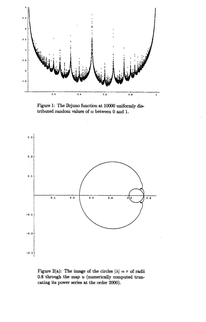
of irrationals. In Figure 1 one can see a plot of the Brjuno functionat 10000

ran-dom values of $a$uniformly distributed in the intervaJ $(0,1)$. Note the logarithmic

singularities associated to each rational number.

6.

Linearization

of

germs

of analytic

diffeomorphisms

Let $\mathbb{C}[[z]]$ denote the ring of formal power series and $\mathbb{C}\{z\}$ denote the ring of

convergent power series.

Let $G$ denote the group of germs of holomorphic diffeomorphi$s\mathrm{m}\mathrm{s}$ of $(\mathbb{C}, 0)$ and let $\hat{G}$

denote the group of formal germs of holomorphic diffeomorphisms of

Small divisors and Brjuno functions

trivialfibrations

$G= \bigcup_{\lambda\in \mathbb{C}}\cdot G_{\lambda}$ $arrow$ $\hat{G}=\bigcup_{\lambda\in \mathbb{C}}\cdot\hat{G}_{\lambda}$

$\pi\downarrow$ $\mathbb{C}^{*}$ where $\hat{\pi}\downarrow$ (6.1) $\mathbb{C}^{*}$ $\hat{G}_{\lambda}=\{\hat{f}(z)=\sum_{n=1}^{\infty}\hat{f}_{n}z^{n}\in \mathbb{C}[[z]],\hat{f}_{1}=\lambda\}$ , (6.2)

$G_{\lambda}= \{f(z)=\sum_{n=1}^{\infty}f_{n}z^{n}\in \mathbb{C}\{z\}, f_{1}=\lambda\}$

.

(6.3)

Let $R_{\lambda}$ dcnotc the germ _{$R_{\lambda}(z)=\lambda z$}. This is the simplest, element of $G_{\lambda}$. It is easy to check that, if A is not a root

of unity, its centralizer is

Cent$(R_{\lambda})=$ $\{R_{\mu}, \mu\in \mathbb{C}"\}$

.

Definition 6.1 A germ $f\in G_{\lambda}$ is linearizable if thcre exists _{$h_{f}\in G_{1}$} (a

linearization of$f$) such that $h_{f}^{-1}fh_{f}=R_{\lambda}$, i.e. $f$ is conjugate to (its linearpart)

$R_{\lambda}$. $f$isformally linearizable ifthere exists$\hat{h}_{f}\in\hat{G}_{1}$ such that_{$\hat{h}_{f}^{-1}f\hat{h}_{f}=R_{\lambda}$} (note

that in this case this is a $f\mathrm{u}$nctional

$e\mathrm{q}$uation in the ring $\mathbb{C}[[z]]$ offormal power series).

When A isa root ofunity it is not difficult to prove thefollowingProposition (see,

e.g. [Ma2]$)$

Proposition 6.2 Assum$e\lambda$ isa primitive root of unity of order

$q.$ A germ$f\in G_{\lambda}$

islineariza$ble$if and only if_$f^{q}=id$. Thesame holds fora formalgerm $\hat{f}\in\hat{G}_{\lambda}$

.

When A is not a root of unity the lincarization (if it exists) is unique and one

can recursively determine the coefficients $h_{n}$ of the power series expansion of

$h_{f}(z)= \sum_{n=1}^{\infty}h_{n}z^{n}$. Indeed $\mathrm{h}\mathrm{o}\mathrm{m}$ the linearization equation

$fh_{f}=h_{f}R_{\lambda}$ we

get, for $n\geq 2$ (remember that we want $h\in G_{1}$, thus $h_{1}=1$) :

$h_{n}= \frac{1}{\lambda^{n}-\lambda}\sum f_{j}n$

$j=2$

Stefano Marmi

In the holomorphic case the problei ofa completeclassification of the conjugacy

classes is open, formidably complicated and perhaps unreasonable [Yo2, $\mathrm{P}\mathrm{M}2$,

$\mathrm{P}\mathrm{M}3]$

.

The first important result in the holomorphic case

is the classical

Koenigs-Poincar\’e Theorem which gives a complete solution to the problem of conjugacy

classes in the hyperbolic case, i.e. when $|\lambda|\neq 1$.

Theorem 6.3 (Koenigs-Poincar\’e) $If|\lambda|\neq 1$ then $G_{\lambda}$ is a conjugacyclass, i.e.

all$f\in G_{\lambda}$ arelinearizable.

Proof.

Since $f$ is holomorphic around $z=0$ there exi$s\mathrm{t}\mathrm{s}c_{1}>1$ and $r\in(0,1)$

such that $|f_{j}|\leq c_{\rceil}r^{1-j}$ for all _{$j\geq 2$}. Since $|\lambda|\neq 1$ there exists _{$c_{2}>1$} such that $|\lambda^{n}-\lambda|^{-1}\leq c_{2}$ for all $n\geq 2$

.

Let $(\sigma_{n})_{n\geq 1}$ be the following recursively defined sequence:

$\sigma_{1}=1,$ $\sigma_{n}=\sum n$

$\sum_{j=2n_{1}+\ldots+n_{j}=n}\sigma_{n_{1}}\cdots\sigma_{n_{j}}$ . (6.5)

The generatingfunction $\sigma(z)=\sum_{n=1}^{\infty}\sigma_{n}z^{n}$satisfies the functional equation

$\sigma(z)=z+\frac{\sigma(z)^{2}}{1-\sigma(z)}$ , (6.6)

thus $\sigma(z)=\frac{1+z-\sqrt{1-6z+z}}{4}$ is analytic in the disk _{$|z|<3-2\sqrt{2}$ and bounded and}

continuous on its closure. By Cauch.y$‘ \mathrm{s}$ estimate

onc

h&s

$\sigma_{n}\leq c_{3}(3-2\sqrt{2})^{1-n}$ for

some $c_{3}>0$

.

Since $\lambda$ is not a root of unity,

$f$ is formally linearizable and the power series

coefficients of its forrnal linearization $\hat{h}_{f}$ sati$s\mathrm{f}\mathrm{y}(6.4)$

.

By induction one$\mathrm{c}\mathrm{a}\iota 1$ check

that $|\hat{h}_{n}|\leq(c_{1}c_{2}r^{-1})^{n-1}\sigma_{n}$, thus $\hat{h}_{f}\in \mathbb{C}\{z\}$

.

$\square$

Remark6.4 Sincethebound $|\lambda^{n}-\lambda|^{-1}\leq c_{2}$ is uniformw.r.t $\lambda\in D(\lambda_{0}, \delta)$, where

$\lambda_{0}\in \mathbb{C}^{*}\backslash \mathrm{S}^{1}$ and $\delta<\mathrm{d}\mathrm{i}\mathrm{s}\mathrm{t}(\lambda_{0}, \mathrm{S}^{1})$, the above given proof of the Poincar\’e-Koenigs

Theorem shows that the map

$\mathbb{C}^{*}\backslash \mathrm{S}^{1}arrow G_{1}$ $\lambdarightarrow h_{\overline{f}}(\lambda)$

is analytic for all $\tilde{f}\in z^{2}\mathbb{C}\{z\}$, where

$h_{\overline{f}}(\lambda)$ is the linearization of $\lambda z+\tilde{f}(z)$.

This notion needs a little comment since $\mathbb{C}\{z\}$ is a rather wild space : it is an

inductive limit of Banach spaces, thus it is a locally convex topological vector

Small divisors and Brjuno functions

Here we simply mean that if$\lambda$ varies in some relatively compact open connected

subset of$\mathbb{C}^{*}\backslash \mathrm{S}^{1}$ then

$h_{\overline{f}}(\lambda)$ belongs to some fixed Banach space of holomorphic

functions (e.g. the Hardy space $H^{\infty}(\mathrm{D}_{r})$ of bounded analytic functions on the

disk $\mathrm{D}_{r}=\{z\in \mathbb{C}, |z|<r\}$, where $r>0$ is fixed and small enough) and depends analytically on $\lambda$ inthe usual sense.

In the next Sections we will concentrate on the study ofthe problem ofexistence

of linearizations of gcrms of holomorpIlic diffcomorphisms. To this purpose thc

following “normalization” will be useful.

Let us note that there is an obvious action of C’ on $G$by homotheties :

$(\mu, f)\in \mathbb{C}^{*}\mathrm{x}Grightarrow$ Ad_{$R_{\mu}f=R_{\mu}^{-1}fR_{\mu}$} . (6.7)

Note that this action leaves the fibers $G_{\lambda}$ invariant. Also, _{$f\in G_{\lambda}$} is linearizable

if and only if Ad$R_{\mu}f$ is also linearizable for all $\mu\in \mathbb{C}^{*}$ (indeed if $h_{f}$ linearizes $f$

then Ad$R_{\mu}h_{f}$, linearizes $\mathrm{A}\mathrm{d}_{R_{\mu}}f$). Therefore, in order to study the problem of the

existence of a linearization, it is enough to consider $G/\mathbb{C}$“, i.e. we identify two

germs of holomorphic diffeomorphisms which are conjugate by a homothety.

Consider thc space $S$ of univalcnt maps $F$ : $\mathrm{D}arrow \mathbb{C}$ such that _{$F(\mathrm{O})=0$} and

the projection

$Garrow S$ $f\mapsto F=\{$

$f$ if$f$ is univalent in$\mathrm{D}$

$\mathrm{A}\mathrm{d}_{R},$$f$ if$f$ is univalent in $\mathrm{D}_{r}$

Thismap is clearlyonto andtwo germshave thesameimageonlyiftheycoincideor

if theyare conjugate bysome homothety. Thus this projection inducesa bijection

from $G/\mathbb{C}^{*}$ onto$S$

.

In what follows wc will always considcr the topological space $S$ of gcrms of

holomorphic diffeomorphisms $f$ : $\mathrm{D}arrow \mathbb{C}$such that _{$f(\mathrm{O})=0$} and _$f$ is univalent in

D. We will denote

$\bullet$ $S_{\lambda}$ the subspace of _$f$ such that $f’(\mathrm{O})=\lambda$;

$\bullet$ $S_{\mathrm{I}}$ the subspace of _$f$ such that $|f’(0)|=1$

.

Clearly the projection above induces a bijection between $G_{\lambda}/\mathbb{C}^{*}$ and $S_{\lambda}$.

To each germ $f\in S,$ $|f’(0)|\leq 1$, one canassociate a natural $f$-invariant compact set

Stefano Marmi Let $U_{f}$ denote the connected cooponent of the interior of $K_{f}$ which contains $0$

.

Then $0$ is stable if and only if $U_{j}\neq\emptyset$, i.e. if and only if$0$ belongs to the interior

of$K_{f}$. Clearly, if$f\in S$and $|f’(0)|<1$ then$0$ is stable.The extremelyremarkable

factis thatstability, whichis atopological property, isequivalentto linearizability,

which is an analytic property.

Theorem 6.5 Let $f\in S,$ $|f’(0)|\leq 1.0$ is stable if and only if$f$ is lineariza$ble$

.

Proof.

The statement is non-trivial only if $\lambda=f’(0)$ has unit modulus. If $f$ is

linearizable then thelinearization$h_{f}$ mapsasmall disk$\mathrm{D}_{r}$ around

zero

conformally

intoD. Since $h_{f}(0)=0$and $|f^{n}(z)|<1$ for all$z\in h_{f}(\mathrm{D}_{r})$ one

sees

that $0$is stable.

Conversely assumc now that $0$ is stable. Then $U_{f}\neq\emptyset$ and onecan casily scc

that it must also be simply connected (otherwise, if it had a hole $V$, surrounding

it with some closed curve $\gamma$ contained in $U_{f}$ since $|f^{n}(z)|<1$ for all $z\in\gamma$ and

$n\geq 0$ the inaximurn principle leads to the

same

conclusionfor all the points in $V$ thus $V\subset U_{f}$). Applying the Riemann mapping theorem to $U_{f}$ one sees that by

conjugation with the Riemann map $f$ induces a univalent map $g$ of the disk into

itselfwith the same linear part $\lambda$. By Schwarz’ Lemma one must have

$g(z)=\lambda z$

thus $f$ is analytically linearizable. $\square$

When $\lambda=f’(\mathrm{O})$ has modulus one, it is not

a

root of unity and $0$ is stable then

$U_{f}$ is conformally equivalent to a disk and is called the Siegel disk of $f$ (at $0$).

Thus the Siegel disk of $f$ is the maxilal connected open set containing $0$ on

which $f$ is conjugated to $R_{\lambda}$. The conformal representation $\tilde{h}_{f}$ :

$\mathrm{D}_{\mathrm{c}(f)}arrow U_{f}$ of $U_{f}$ which satisfies $\tilde{h}_{f}(0)=0,\tilde{h}_{f}’(0)=1$ linearizes $f$ thus the power series of $\tilde{h}_{f}$

and $h_{f}$ coincide. If $r(f)$ denotes the radius of convergence of the linearization $h_{f}$ (whose power meries coefficients are recursively determined as in (6.4)),

we

see that $c(f)\leq r(f)$. One can prove that $c(f)=r(f)$ when at _least one of _{the two}

following conditions is satisfied : (i) $U_{f}$ is relatively compact in $\mathrm{D}$;

(ii) each point of$\mathrm{S}^{1}$ is asingularity of

$f$.

7. Small divisors

When $|\lambda|=1$ and $\lambda$ is not aroot of unity we canwrite

$\lambda=e^{\mathit{2}\pi i\alpha}$ with

$\alpha\in \mathbb{R}\backslash \mathbb{Q}\cap(-1/2,1/2)$ ,

and whether $f\in G_{\lambda}$ is linearizable or not depends crucially on the arithmetical

Small divisors and Brjuno functions

look atthelinearization problem asthe problem ofdeciding if quasiperiodicorbits

are_{preserved (locally) under analytic perturbation. This isnot always thecase as}

thefollowing simple Theorem shows :

Theorem 7.1 (Cremer) If $\lim\sup_{narrow+\infty}|\{n\alpha\}|^{-1/n}=+\infty$ then there exists

$f\in G_{e^{2\pi:\alpha}}$ which is not $lin$earizablc.

Proof.

First of all note that $\lim\sup_{narrow+\infty}|\{n\alpha\}|^{-1/n}=+\infty$ if and only if

$\lim_{narrow+}\sup_{\infty}|\lambda^{n}-1|^{-1/n}=+\infty$

since

$|\lambda^{n}-1|=2|\sin(\pi n\alpha)|\in(2|\{n\alpha\}|, \pi|\{n\alpha\}|)$ .

Then we construct $f$ in the following manner: for $n\geq 2$ we take $|f_{n}|=1$ and we

choose inductively $\arg f_{n}$ such that

$\arg f_{n}=\arg\sum f_{j}n-1$

$j=2$

$\sum_{n_{1}+\ldots+n_{j}=n}\hat{h}_{n_{1}}\cdots\hat{h}_{n_{j}}$ , (7.1) (recall the inductionformula (6.4) _{for the coefficients}of the formal linearizationof

$f$ and notc that the r.h.s. of (7.1) is a polynomial in $n-2$ variables $f_{2},$

$\ldots,$$f_{n-1}$

with coefficients in the field $\mathbb{C}(\lambda))$

.

Thus

$| \hat{h}_{n}|\geq\frac{|f_{n}|}{|\lambda^{n}-1|}=\frac{1}{|\lambda^{n}-1|}$

and $\lim\sup_{narrow+\infty}|\hat{h}_{n}|^{1/n}=+\infty$ : the formal linearization $\hat{h}$

is a divergent series.

$\square$

Clearly the set of irrational numbers satisfying the assumption of Cremer’s

Theorem is a dense $G_{\delta}$ withzero Lebesgue

measure.

Aftcrthis negative result, it waspretty clearthattheproblcmoftheexistence

of analyticlinearizations was not an easy one. The main difficultyis given by the

unavoidable presence of small divisors in the

recurrence

(6.4). This difficulty

was

flrst overcomc by Siegel in 1942 [S] but it was clearly well-known among

mathematicians at $t$he end of the 19th and at the beginning ofthe 20th century.

Assume that $a\in$ CD$(\tau)$ for

some

$\tau\geq 0$

.

Recalling the

recurrence

(6.4) for

the power series coefficients ofthe linearization oneseesthat $h_{n}$ isapolynomial in

$f_{2},$

$\ldots,$$f_{n}$ with coefficients whicharerationalfunctionsof$\lambda:h_{n}\in \mathbb{C}(\lambda)[f_{2}, \ldots, f_{n}]$

Stefano Marmi

Let us compute explicitely the first few terms of the

recurrence

$h_{2}=(\lambda^{2}-\lambda)^{-1}f_{2}$ ,

$h_{3}=(\lambda^{3}-\lambda)^{-1}[f_{3}+2f_{2}^{2}(\lambda^{2}-\lambda)^{-1}]$ ,

$h_{4}=(\lambda^{4}-\lambda)^{-1}[f_{4}+3f_{3}f_{2}(\lambda^{2}-\lambda)^{-1}+2f_{2}f_{3}(\lambda^{3}-\lambda)^{-1}$ (7.2) 4$f_{2}^{3}(\lambda^{3}-\lambda)^{-1}(\lambda^{2}-\lambda)^{-1}+f_{2}^{3}(\lambda^{2}-\lambda)^{-2}]$ ,

and soon. Itisnot difficult to seethat among all contributes to $h_{n}$ there isalways

aterm of the form

$2^{n-2}f_{2}^{n-1}[(\lambda^{n}-\lambda)\ldots(\lambda^{3}-\lambda)(\lambda^{2}-\lambda)]^{-1}$ (7.3)

If one then tries to estimate $|h_{n}|$ by simply summing up the absolute values of

each contribution then one term will bc

$2^{n-2}|f_{2}|^{n-1}[|\lambda^{n}-\lambda|\ldots|\lambda^{3}-\lambda||\lambda^{2}-\lambda|]^{-1}\leq 2^{n-2}|f_{2}|^{n-1}(2\gamma)^{(n-1)\tau}[(n-1)!]^{\tau}(7.4)$

if$a\in$ CD$(\gamma, \tau)$ and

one

obtains a divergent bound. Note the differencewith the

case $|\lambda|\neq 1$ : in thi$s$ case thebound would be $|\lambda|^{-(n-1)}2^{n-2}|f_{2}|^{n-1}c^{n-1}$ for some

positive constant $c$ independent of$f$. Thus onemust use a more subtle majorant

series method.

The key point is that the estimate (7.4) is far too pessimistic : indeed ifone

considers the generating series associated to the small denominators appearing in

the terms (7.3) ($\mathrm{i}.\mathrm{c}$. the scries

$\sum_{n=1rightarrow^{z^{n}}(\lambda-1}^{\infty}(\lambda^{n}-1)$ one can evcn provc [HL] that

it haspositive radius ofconvergence whenever$\lim\sup_{narrow\infty}\frac{\log q_{k\mathrm{I}1}}{q_{k}}<+\infty$.

8.

The

quadratic

polynomial and

Yoccoz’s

ftnction

Inthis Section we will study in detail the linearizationproblem for the quadratic

polynomial

$P_{\lambda}(z)= \lambda(z-\frac{z^{2}}{2})$ (8.1)

Apart from being the simplest nonlinear map, one good reason for starting our

investigations from $P_{\lambda}$ is provided by a theorem ofYoccoz [Yo2, pp.59-62] which

shows how the quadratic polynomial is the “worst possible perturbation of the linear part $R_{\lambda}$” as the following statement makes precise:

Small divisors and Brjuno functions

Theorem 8.1 Let $\lambda=e^{2\pi i\alpha},$ $\alpha\in \mathbb{R}^{\backslash }\backslash \mathbb{Q}$

.

If$P_{\lambda}$ is linearizable then every germ $f\in G_{\lambda}$ is also linearizable.

The previous Theorem shows that the linearizability of the quadratic polynomial for a certain $\lambda$ implies that

$G_{\lambda}$ is a conjugacy class. On the other hand one can

prove thefollowing

Theorem 8.2 Let $\lambda=e^{2\pi i\alpha}$,

$a$ $\in \mathbb{R}\backslash$Q. For almost all $\lambda\in \mathrm{T}$ the quadratic

polynomial $P_{\lambda}$ is lineariza$bl\mathrm{e}$.

In 1942 C.L. Siegel [S] proved that all analytic germs $f\in G_{\lambda}$ with $a\in$ CD

are analytically linearizable, thus showing a more precise andmore general result

than Theorem 8.2. Siegel’s result, later improved by Brjuno [Br], is based on a

very clever and careful control of the accumulation ofsmall denominators in the

nonlinear

recurrence

(6.4). Here however we want to follow a different approach

and wcwill sketch an argument, again due to Yoccoz, which does not makeuse of any small denominators estimates.

The quadratic polynomial $P_{\lambda}$ has a unique critical point $c=1$ with

corre-sponding critical value $v_{\lambda}=P_{\lambda}(c)=\lambda/2$. If$|\lambda|<1$ by Koenigs-Poincar\’e theorem

weknow that there exists

a

uniqueanalytic linearization $H_{\lambda}$ of$P_{\lambda}$ and that it

de-pendsanalyticallyon $\lambda$ as$\lambda$varies in D. Let

$r_{2}(\lambda)$ denote the radiusofconvergence of$H_{\lambda}$. One has the following

Proposition 8.3 Let $\lambda\in$ D. Then:

(1) $r_{2}(\lambda)>0$;

(2) $r_{2}(\lambda)<+\infty$ and $H_{\lambda}$ has a continuous extension to$\overline{\mathrm{D}_{r_{2}(\lambda)}}$

.

Moreover the map $H_{\lambda}$ : $\overline{\mathrm{D}_{r_{2}(\lambda)}}arrow \mathbb{C}$ is conformal and verifies

$P_{\lambda}\mathrm{o}H_{\lambda}=H_{\lambda}\mathrm{o}R_{\lambda}$.

(3) On itscircle ofconvergence $\{z, |z|=r_{2}(\lambda)\},$ $H_{\lambda}h$as a $\mathrm{u}$niquesingu$lar$point

which will be denoted$u(\lambda)$.

(4) $H_{\lambda}(u(\lambda))=1$ and $(H_{\lambda}(z)-1)^{2}$ is holomorphic in $z=u(\lambda)$

.

Proof.

The first assertion is just a _{consequence of Koenigs-Poincar\’e theorem.}

The functional equation $P_{\lambda}(H_{\lambda}(z))=H_{\lambda}(\lambda z)$ is satisfied for all $z\in \mathrm{D}_{r_{2}\langle\lambda)}$

.

Moreover $H_{\lambda}$ : $\mathrm{D}_{r_{2}(\lambda)}arrow \mathbb{C}$ is univalent (ifone had $H_{\lambda}(z_{1})=H_{\lambda}(z_{2})$ with $z_{1}\neq z_{2}$

and $z_{1},$ $z_{2}\in \mathrm{D}_{r_{2}(\lambda)}$ one would have $H_{\lambda}(\lambda^{n}z_{1})=H_{\lambda}(\lambda^{n}z_{2})$ for all _{$n\geq 0$} which is

impossible since $|\lambda|<1$ and $H_{\lambda}’(0)=1)$. Thus $r_{2}(\lambda)<+\infty$. On the other hand if $H_{\lambda}$ is holomorphic in $\mathrm{D}_{r}$ for some $r>0$ and the critical value

$v_{\lambda}\not\in H_{\lambda}(\mathrm{D}_{r})$

Stefano Marmi Therefore there exists $u(\lambda)\in \mathbb{C}$ such that $|u(\lambda)|=r_{2}(\lambda)$ and $H_{\lambda}(\lambda u(\lambda))=v_{\lambda}$

.

Such a $u(\lambda)$ is unique since $H_{\lambda}$ is injective on

$\mathrm{D}_{r_{2}(\lambda)}$

.

If $|w|=|\lambda|r_{2}(\lambda)$ and $w\neq\lambda u(\lambda)$ one has $H_{\lambda}(w)=P_{\lambda}(H_{\lambda}(\lambda^{-1}w))$ and

$H_{\lambda}(\lambda^{-1}w)=1-\sqrt{1-2\lambda^{-1}H_{\lambda}(w)}$ (8.2)

which shows how to extend continuously and injectively $H_{\lambda}$ to $\overline{\mathrm{D}_{r_{2}(\lambda)}}$

.

By

construction thefunctional equationistriviallyverified. This completes theproof

of(2).

To prove (3) and (4) note that $\mathrm{h}\mathrm{o}\mathrm{m}H_{\lambda}(\lambda u(\lambda))=P_{\lambda}(H_{\lambda}(u(\lambda)))$it follows

that $H_{\lambda}(u(\lambda))=1$

.

Formula (8.2) shows that all points $z\in \mathbb{C},$ $|z|=r_{2}(\lambda)$

are

regularexcept for $z=u(\lambda)$

.

Finallyonehas $(H_{\lambda}(z)-1)^{2}=1-2\lambda^{-1}H_{\lambda}(\lambda z)$ which

is holomorphic also at $z=u(\lambda)$ , $\square$

The fact that $H_{\lambda}$ is injectivc on $\overline{\mathrm{D}}_{r_{2}(\lambda)}$ implies that $r_{2}(\lambda)<+\infty$. One can easily

obtain a more precise upper bound by

means

of Koebe 1/4-Theorem and prove

that $r_{2}(\lambda)\leq 2$

.

The use of further standard distorsion estimates for univalent

functions allows to prove that the sequence of polynomials $u_{n}(\lambda)=\lambda^{-n}P_{\lambda}^{n}(1)$

converges uniformly to $u$ on compact subsets of D. Thus $u$ : $\mathrm{D}^{*}arrow \mathbb{C}$ has a

bounded analytic extension to $\mathrm{D}$ and _{$u(\mathrm{O})=1/2$}

.

The polynomials

$u_{n}$ verify the

recurrence

relation

$u_{0}(\lambda)=1$ , $u_{n+1}( \lambda)=u_{n}(\lambda)-\frac{\lambda^{n}}{2}(u_{n}(\lambda))^{2}$ (8.3)

The function $u$ : $\mathrm{D}arrow \mathbb{C}$ will be called Yoccoz’s

function.

It has many

remarkable properties and it is the object of various conjectures (see Section 11).

Using (8.3) it is easy to check that $u(\lambda)\in \mathbb{Q}\{\lambda\}$ and all the denominators

are

a

power of 2. Moreover $u(\lambda)-u_{n}(\lambda)=\mathrm{O}(\lambda^{n})$ thus one can also compute the first

terms of the power seriesexpansion of$u$ :

$u( \lambda)=\frac{1}{2}-\frac{\lambda}{8}-\frac{\lambda^{2}}{8}-\frac{\lambda^{3}}{16}-\frac{9\lambda^{4}}{128}-\frac{\lambda^{5}}{128}-\frac{7\lambda^{6}}{128}+\frac{3\lambda^{7}}{256}-\frac{29\lambda^{8}}{1024}-\frac{\lambda^{9}}{256}+\frac{25\lambda^{10}}{2048}+\frac{559\lambda^{11}}{32768}+\ldots$

.

It is easy and fast to compute on

a

personal computer the first

2000

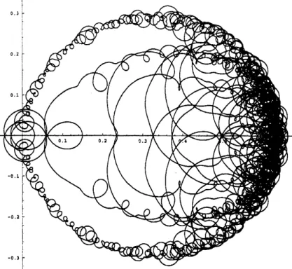
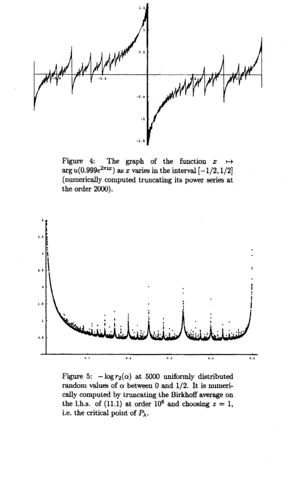
terms of

the seriesexpansionof$u$ : in the Figures$2\mathrm{a}$to $2\mathrm{d}$ one can seetheimagesthrough

$u$

of the circlcs of radii0.8, 0.9, 0.99 and0.999. Figures 3and 4show respectivelythc

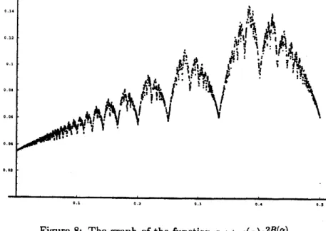
graphofthefunction$xrightarrow|u(0.999e^{2\pi ix})|$ as$x$variesinthe interval $[0,1/2]$ andthe

graph of$x\mapsto\arg u(0.999e^{2\pi ix})$ as $x$ varies in the interval $[-1/2,1/2]$

.

Note that

the argument of the function$u$ seems tohave a decreasingjump ofapproximately

$\pi/q$ at each rational number$p/q$. We refer to [BHH, Ca] for a detailed_numerical

Small _{divisors and Brjuno functions}

We cannow conclude the proofofTheorem 8.2. Let $\lambda_{0}\in \mathrm{T}$ and

assume

that

$\lambda_{0}$ is not a root of unity.

Then on can check easily that

$r_{2}( \lambda_{0})\geq\lim_{\mathrm{D}\ni\lambdaarrow}\sup_{\lambda_{0}}|u(\lambda)|$ (8.4)

but much more can be proved [Yo2, pp. 65-69]

Proposition 8.4 For all$\lambda_{0}\in \mathrm{T},$ $|u(\lambda)|$ has a $no\mathrm{n}-tange\mathrm{n}tial$ limit in $\lambda_{0}$ which is

equal to the radius of

convergence

$r_{2}(\lambda_{0})$ of$H_{\lambda_{0}}$.

Ofcourse, if$\lambda_{0}$ is a $\mathrm{r}\mathrm{o}\mathrm{o}\mathrm{t}_{1}$ of unity then

$P_{\lambda_{0}}$ is not even formally linearizable and

one poses $r_{2}(\lambda_{0})=0$

.

Applying Fatou’s Theorem on the existence and almost everywhere

non-vanishing of non-tarlgential boundary values of bounded holomorphic functions

on the unit disk to $u$ : $\mathrm{D}arrow \mathbb{C}$ one finds that there exists

$u^{*}\in L^{\infty}(\mathrm{T}, \mathbb{C})$ such

that for almost all $\lambda_{0}\in \mathrm{T}$ one has _{$|u^{*}(\lambda_{0})|>0$} and _{$u(\lambda)arrow u(\lambda_{0})$} as

$\lambdaarrow\lambda_{0}$

non tarigentially. From (8.4) one concludes that for almost all $\lambda_{0}\in \mathrm{T}$ one has

$r_{2}(\lambda_{0})>0$. $\square$

9.

_{Renormalization}

_{and quasiperiodic orbits: Yoccoz’s}

_theorems

The ideaofrenormalization has beenextremely successful in dynamics. It$s$origin

is in statistical physics and quantum field theory.

In physics two approaches _{to renormalization} coexist : one (and the oldest)

is perturbative the other is non-perturbative. The lattergrew up from the study of critical phenomena (ferromagnetism, superfluidity, polymers, conductivity of

random media, etc.) and statistical physics. Here one observesthat very different

systems are surprisingly similar in a quantitative way, since they have the same

critical exponents scaling laws (universality). At the critical transition these systems _{are somehow dominated by large distance correlations which}

_are

_not

sensitive to the _{dctails of the microscopic interactions.}

Theapplications_{in dynamical systems of this secondapproachhave been most}

successful. In this Section wewill illustrat$e$ how

one can

rigorously prove optimal

resultsfor the problem oflinearizationof holomorphic germs usinga(geornetrical)

renormalization approach. Otherrigorousresults have been obtained for the local

and global conjugacy problems _{for analytic diffeomorphsism of the circle} [Yo3].

In addition a number of heuristic $\mathrm{r}$esults [CJ, Da2, $\mathrm{M}\mathrm{K}$] have been obtained for

Hamiltonian systems with one frequency (area-preservingmaps ofthe plane or of

Stefano Marmi

The basic idea of (non-perturbative) renormalization in studying

quasiperi-odic orbits is as follows : given our dynamical system $f\in \mathrm{E}\mathrm{n}\mathrm{d},$$(X)$ if it has some

region $X_{0}$ of phase space filled by quasiperiodic orbits then its iterates form an

equicontinuous family on it and $f^{n_{j}+1}\approx f$ for

some

sequence

$n_{j}arrow\infty$

.

Thus one

can

look for aregion $U_{0}\subset X_{0}$ whichreturns (at least approximately) to itself

under$n_{1}$ iterations of$f$. Ifwe thenconstruct the quotient _{$X_{1}=U_{0}/f$} identifying

$x\in U_{0}$ with $f(x)$ the renormalized map$\mathcal{R}_{n_{1}}f\in \mathrm{E}\mathrm{n}\mathrm{d},$ $(X_{1})$ will beinduced by the

first return map to $U_{0}$ (under the iteration of $f$). Thcn $f$ will have quasiperiodic

orbits of frequency $a_{0}\in(0,1)$ if and only if $R_{n_{1}}f$ has quasiperiodic orbits of

frequency $\alpha_{1}$ with$\alpha_{0}^{-1}=\alpha_{1}+n_{1}$.

The process can be iterated. Ifone can control the sequence $\mathcal{R}_{n_{f}}\cdots \mathcal{R}_{n_{1}}f\in$

End, $(X_{j})$ (and the geometriclimit$X_{0}arrow X_{1}arrow X_{2}arrow\ldots$)provingitsconvergence

to some fixed point $f_{\infty}\in$ End,$(X_{\infty})$, where $X_{\infty},$ _{$= \lim X_{j}$} then one has proved

that the dynamics of $f$ on $X_{0}$ is the

same

as the dynamics of $f_{\infty}$ on $X_{\infty}$. In

the quasiperiodic case $f_{\infty}$ typically is a linear automorphism of

$X_{\infty}$ (trivial fixed point) but other possibilities

are

conceivable.

In what follows we will very briefly and _{approximately describe Yoccoz’s} analysisofthc rcnormalization of quasiperiodic orbits in the simplest caseof Sicgel

domains.

A qualitative analysis of the $\mathrm{b}\mathrm{a}s$ic construction (first

return map and geometric

quotient) alreadygives some non-trivialinformation on the dynamics ofgerms of

holomorphic diffeomorphisms with an indifferent fixed point.

Let $\mathcal{Y}$ denote the set of _$a$ $\in \mathbb{R}\backslash \mathbb{Q}$ such that all holomorphic germs of

diffeomorphisrnsof $(\mathbb{C}, 0)$ withlinear part $e^{2\pi i\alpha}$ are

linearizable. The results of thc

previous Section show that $\mathcal{Y}$ has full

measure

(combine Theorems 8.1 and

8.2) butits complement in $\mathbb{R}\backslash \mathbb{Q}$is a$G_{\delta}$-dense (Theorem 7.1). Further informationon

the structureof$\mathcal{Y}$ is provided by the following

Theorem 9.1 $(\mathrm{D}\mathrm{o}\mathrm{u}\mathrm{a}\mathrm{d}\mathrm{y}-\mathrm{G}\mathrm{h}\mathrm{y}s)\mathcal{Y}$is _{$SL(2, \mathbb{Z})$}-invariant.

Proof.

(sketch). $\mathcal{Y}$ is clearly invariant under $T$, thus we

only need to show that if

$\alpha\in \mathcal{Y}$ then also $U\cdot a=-1/\alpha\in \mathcal{Y}$.

Let $f(z)=e^{2\pi i\alpha}z+\mathrm{O}(z^{2})$ and consider a dornain $V’$ bounded by

1) a segment $l$ joining $0$ to $z_{0}\in \mathrm{D}$“, $l\subset \mathrm{D}$;

2) its image $f(l)$ ;

3) a

curve

$l’$joining

$z_{0}$ to $f(z_{0})$.

We choose $l’$ and

$z_{0}$ (sufficiently close to $0$) so that $l,$ $l’$ and _$f(l)$ do not intersect

Small divisors and Brjuno functions

Then glueing $l$ to $f(l)$ one

obtains a topological manifold $\overline{V}$ with boundary

which is homeomorphic to $\overline{\mathrm{D}}$

. With the induced complex structure its interior is

biholomorphic to D. Let us nowconsiderthe

_first

retum map$g_{V’}$ to thedomain$V$‘

(this is welldefinedif$z$ischoosenwith$|z|$ small enough) : if$z\in V’$ (and $|z|$issmall

enough) we define $g_{V’}(z)=f^{n}(z)$ where $n$ (depends on

$.z$) is defined asking that

$f(z),$$\ldots,$$f^{n-1}(z)\not\in V’$ and $f^{n}(z)\in V’$, i.e. $n= \inf\{k\in \mathrm{N}, k\geq 1, f^{k}(z)\in V’\}$.

Then it is easy to check that $n=[ \frac{1}{\alpha}]$ or $n=[ \frac{1}{\alpha}]+1$

.

The first return map _{$g_{V’}$}

inducesamap$\mathit{9}_{\overline{V}}$onaneighborhoodof

$0\in\overline{V}$ and finallya germ

$g$ofholomorphic

diffeomorphism at $\mathrm{O}\in \mathrm{D}(gp=pg_{\overline{V}}$, where _$p$ is the projection $\mathrm{h}\mathrm{o}\mathrm{m}\overline{V}$to

the disk

D). It is easy to check that $g(z)=e^{-2\pi i/\alpha}z+\mathrm{O}(z^{2})$ (note that in the passage

from $V’$ to $\mathrm{D}$ through $\overline{V}$

the angle $2\pi\alpha$ at the originis rnapped in $2\pi$).

To eachorbit of$f$ near $0$ corresponds an orbit of

$g$ near $0$. In particular

$\bullet$ $f$ is linearizable ifand only if

$g$ is linearizable;

$\bullet$ if$f$ has a periodic orbit near $0$ then also

$g$ has a periodic orbit;

$\bullet$ if_$f$hasapoint ofinstability (i.e. apointwhose iterates leave

aneighborhood of $0$) then also 9 has a point of instability (which will escape even more

rapidly).

In particular thesc statements showthat $a\in \mathcal{Y}$ if and only $\mathrm{i}\mathrm{f}-1\oint\alpha\in \mathcal{Y}$. $\square$

We willnow_{briefly describe how to turn the above construction into aquantitative}

construction and how to use it to give a artihmetical characterization of the set

$\mathcal{Y}$ : it will turn out that it coincides with tlle set of Brjuno nurnbers.

Let$S(\alpha)$ denotethe universal cover of$S_{\mathrm{e}^{2n\dot{\mathrm{t}}\alpha}}$

.

An element$F\in S(\alpha)$ is a umivalent

function $F$ : $\mathbb{H}arrow \mathbb{C}$ and _{$F(z)=z+\alpha+\varphi(z)$} where

$\varphi$ is -periodic and

$\lim_{\Im mzarrow+\infty}\varphi(z)=0$. Let $E$ : $\mathbb{H}arrow \mathrm{D}^{*}$ be the cxponential map _{$E(z)=e^{2\pi iz}$} :

each function $f\in S_{\mathrm{e}^{2\pi\cdot\alpha}}$ lifts to such a map $F$ and $E\mathrm{o}F=f\mathrm{o}E$.

Let $r>0,$ $\mathbb{H}_{r}=\mathbb{H}+ir$

.

It is clear that if _{$F\in S(a)$} and $r$ is sufficiently large

then $F$ is very close to the translation _{$zrightarrow z+\alpha$} for $z\in \mathbb{H}_{r}$. Indeed using the compactnessofthespace$S(\alpha)$ and the distorsion estimates for univalent functions

one

canprove the following:

Proposition 9.2 Let $\alpha\neq 0$. There exists a universal constant _{$c_{0}>0$} (i.e.

independent ofa) such that for all $F\in S(\alpha)$ and for all$z\in \mathbb{H}_{t(\alpha)}$ where

$t(a)= \frac{1}{2\pi}\log\alpha^{-1}+c_{0}$ , (9.1)

one $h$as

Stefano Marmi

Given $F$, the lowest admissible value $t(F, \alpha)$ of $t(\alpha)$ such $\mathrm{t}\}_{1\mathrm{a}}\mathrm{t}(9.2)$ holds for all

$z\in \mathbb{H}_{t(F,\alpha)}$ represents the height in the upper half plane $\mathbb{H}$ at which the strong

nonlinearities of$F$ manifest themselves. When _{$\Im mz>t(F, \alpha),$} $F$ is very close to

thetranslation $T_{\alpha}(z)=z+\alpha$. This is equivalent to saythat $f$ isvery close to the

rotation by $2\pi a$ when $z\in \mathrm{D}$ issufficiently small.

Anexampleofstrong nonlinearity is ofcourse a fixedpoint : if$F(z)=z+\alpha+$

$\frac{1}{2\pi i}e^{2\pi iz},$ $\alpha>0$, then$z=- \frac{1}{4}+\frac{1}{2\pi}\log(2\pi\alpha)^{-1}$isfixed and $t(F, \alpha)\geq\frac{1}{2\pi}\log(2\pi\alpha)^{-1}$.

Following theconstruction in the proof ofDouady-Ghysthcoremwecan now

consider the first return map in the “strip” $B$ delimited by _{$l=[it(\alpha),$}$+i\infty[$

,

$F(l)$ and the segment [it$(\alpha),$$F(it(\alpha))$]. Given $z$ in $B$

we

can iterate $F$ until

$\Re eF^{n}(z)>1$. If $\Im mz\geq t(\alpha)+c$ for some $c>0$ then _{$z’=F^{n}(z)-1\in B$}

and $z-\rangle$ $z’$ is the first return map in the strip $B$. Glueing $l$ and $F(l)$ by _$F$ one

obtains a Riemann surface $S$ corresponding to int$B$ and biholomorphic to $\mathrm{D}^{*}$

.

This induces a map $g\in S_{e^{2\pi i/\alpha}}$ which lifts to $G\in S(\alpha^{-\infty})$.

As we can

see

we have three steps :

(g) glueing $l$ and $F(l)$ following _$F$ we get a

topological manifold with boundary

whose interioris biholomorphic to the standard half-cylinder;

(u) uniform,ization of the manifold obtaining a standard cylinder;

(d) developing the standard cylinder

on

the plane.

The biholomorphism $H=d\mathrm{u}g$ which “glues, uniformizes and develops” the

“strip” $B$ into thc strip of width 1 conjugatcs $F$ with thc translation by 1 $H(F(z))=H(z)+1$

and the renormalized map is

$G=\mathcal{R}_{a_{1}}F=HF^{a_{1}}T_{-1}H^{-1}$ ,

where $a_{1}$ is the integer part of $\alpha^{-}$

‘i.

It isimmediate to checkthat if$\Im mz$ is large

then $H(z)= \frac{z}{\alpha}+\ldots$ and one can then show the following (see [Yo2], pp. 32-33)

Proposition 9.3 Let $\alpha\in(0,1),$ $F\in S(\alpha)$ and$t(a)>0$ such that if$\Im mz\geq t(\alpha)$

$thcn|F(z)-z-\alpha|\leq\alpha/4$. Thcre exists$G\in S(\alpha^{-1})$suchthatif$z\in \mathbb{H},$ $\Im mz\geq t(\alpha)$

and $F^{:}(z)\in$ IHf for all $i=0,1,$

$\ldots,$$n,$ $-1$ but $F^{n}(z)\not\in \mathbb{H}$ then there exists $z’\in \mathbb{C}$

such that

1. $\Im mz’\geq\alpha^{-1}(\Im_{7}nz-t(a)-c_{1})$, where $c_{1}>0$ is a universal constan$t$;

2. There exists an integer$m$ such that $0\leq m<n$ and $G^{m}(z’)\not\in$IHI.

Small divisors and Brjuno functions

CLAIM :

_If

$\alpha$ is a Brjuno number the $reno7malization$ scheme converges and all

maps $f\in S_{e^{2\pi\cdot\alpha}}$ are linearizable.

If $F\in S(\alpha)$ is a lift of $f\in S_{e^{2\pi \mathrm{t}\alpha}}$, let $K_{F}\subset \mathbb{C}$ be defined as the cover of _{$K_{f}$} :

$E(K_{F})=K_{f}$

.

It is immediat$e$ tocheck that

$d_{F}= \sup\{smz\triangleright|z\in \mathbb{C}\backslash K_{F}\}=-\frac{1}{2\pi}\log$ dist$(0, \mathbb{C}\backslash K_{f})$ . (9.3)

An upper bound ofthe form

$\sup d_{F}\leq\frac{1}{2\pi}B(a)+C$ _(9.4)

$F\in S(\alpha)$

for some universal constant $C>0$ _{is therefore enoughto establish our claim.}

Assume that (9.4) is not true and that there exist a $\in \mathbb{R}\backslash \mathbb{Q}\cap(0,1/2)$ with

$B(\alpha)<+\infty,$ _{$F\in S(a),$} $z\in \mathbb{H}$ and $n>0$ such that $\Im mF^{n}(z)\leq 0$ ,

$\Im mz\geq\frac{1}{2\pi}B(\alpha)+C$ .

Let

us

choose $\alpha,$ $F$ and $z$

so

that $n$ is

as

small as possible. By Proposition

9.3, if$C>c_{0}$, one gets

$\Im mz’\geq\alpha^{-1}[\Im mz-t(\alpha)-c_{1}]$

$\geq a^{-1}[\frac{1}{2\pi}(B(\alpha)-\log\alpha^{-1})+C-c_{0}-c_{1}]$

By the functional equation of$B$ one gets

$\Im mz’\geq\frac{1}{2\pi}B(\alpha^{-1})+a^{-1}[C-c_{0}-c_{1}]\geq\frac{1}{2\pi}B(\alpha^{-1})+C$

provided that $C\geq 2(c_{0}+c_{1})$

.

But Proposition 9.3shows that this contradicts the

minimality of$n$ and we must therefore conclude that (9.4) holds. $\square$

Yoccoz has bcen able to cstablish also alowcr bound

$\inf_{F\in S(\alpha)}d_{F}\geq\frac{1}{2\pi}B(\alpha)+C$ (9.5)

again using the renormalization construction together with some analytic surgery

so as to be able at each step of the renormalization constructionto glue a fixed

Stefano Marmi

proof ofthis lower $\mathrm{b}\mathrm{o}\mathrm{u}\iota \mathrm{l}\mathrm{d}$ can be found

in the Bourbaki seminar ofRicardo

Perez-Marco [PM1].

10.

Stability of

quasiperiodic

orbits

in

one-frequency systems

:

rigorous results

The main result of the renormalization analysis made by Yoccoz of the problem

of linearization ofholomorphic germs of $(\mathbb{C}, 0)$ can bevery simply stated as

$\mathcal{Y}=\{\alpha\in \mathbb{R}\backslash \mathbb{Q}|B(\alpha)<+\infty\}=\mathrm{B}\mathrm{r}\mathrm{j}\mathrm{u}\mathrm{n}\mathrm{o}$ numbers,

but he proves much more than the above.’

Theorem 10.1

$(a)$ If$B(\alpha)=+\infty$ there existsa $non-l\mathrm{i}ne\mathrm{a}riz\mathrm{a}ble$ germ _{$f\in S_{e^{2\pi 1\propto j}}$}

(b) If$B(a)<+\infty$ then $r(\alpha)>0$ and

$|\log r(\alpha)+B(\alpha)|\leq C$, (10.1)

where $C$ is a universalconstant (i.e. independent of$\alpha$);

$(c)$ Let $\lambda=e^{2\pi i\alpha}$ and consider the Yoccoz function

$u$ defined in Section 8. Recdl

that $|u(\lambda)|=r_{2}(\lambda)$, i.e. the radius of convergence of the linearization of the quadratic polynomial. There exists a universal constant $C_{1}>0$ such that for

all Brjuno numbers $a$ one has

$B(\alpha)-C_{1}\leq-\log|u(\lambda)|\leq B(\alpha)+C_{1}$ . (10.2)

Notc that thc upper bound in (c) was proved in [Yol] togcther with a weakcr

lower bound : this version of (c) is actually due to to X. Buff and A. Ch\’eritat

[BC1]. Results similar to Theorem 10.1 hold for the local conjugacy of analytic

diffeornorphisms of the circle [Yol, Yo3] and for

sorne

$\mathrm{a}\mathrm{r}\mathrm{e}\mathrm{a}-\mathrm{p}\mathrm{r}e\mathrm{s}\mathrm{e}\mathrm{r}\mathrm{v}\mathrm{i}\mathrm{n}\mathrm{g}$ maps

[Mal,Dal], including the standard family [Da2, BGI, $\mathrm{B}\mathrm{G}2$].

Theremarkable consequence of (10.1) and (10.2) is that the Brjuno function

not only identifies the set $\mathcal{Y}$ but also gives a rather precise estimate of the sizeof

the Siegel disks.

The first open problemwe want to address is whether or not the infimum in (10.1) is attained by the quadratic polynomial $P_{\lambda}(z)= \lambda z(1-\frac{z}{2})$ :

Question 10.2 Does $r(\alpha)=$ inf$f\in s_{\mathrm{e}^{2\pi\cdot\alpha}}r(f)=r_{2}(e^{2\pi}):\alpha$, i.e. the radius of