Volume conjecture for various quantum $SO(3)$ invariants (Topology and Analysis of Discrete Groups and Hyperbolic Spaces)
16
0
0
全文
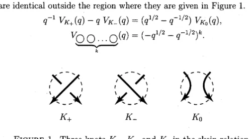
(2) 109. are identical outside the region where they are given in Figure 1.. q^{-1} V_{K+}(q)-qV_{K_{-}}(q)=(q^{1/2}-q^{-1/2})V_{K_{0}}(q). ,. V q)=(-q^{\mathrm{i}/2}-q^{-1/2})^{k}. K_{+} K_{-} K_{0} FIGURE 1. Three knots. K_{+},. K_{-} and. K_{0} in the skein relation. The Jones polynomial is also constructed by the quantum R ma‐ trix corresponding to the vector representation of the quantum group \mathcal{U}_{q}(sl_{2}) . This construction is easily generalized to any irreducible rep‐ resentation of any quantum group obtained from a semisimple Lie alge‐ bra. The invariant coming from an irreducible representation of \mathcal{U}_{q}(sl_{2}) is called the colored Jones invariant, which is denoted by V_{K}^{(l)}(q) , where l is the dimension of the corresponding representation. For a link L whose components are L_{1}, L_{2}, , L_{p} , we also have the colored \cdots. Jones invariant V_{L}^{(t_{1},l_{2},\cdots,l_{p})}(q) where the component L_{j} is attached by the l_{j} dimensional representation. Let M be a closed 3 manifold given by the surgery along a framed link L=L_{1}\cup L_{2}\cup\cdots\cup L_{p} \subset S^{3} . Then, for a positive integer r , the Witten‐Reshetikhin‐Turaev invariant $\tau$^{(r)}(M) is given by the following.. \displayst le\overline{$\tau$}^{(r)}(M)=\sum_{l 1}=1}^{r-1} \displayst le\sum_{l p}=1^{r-1}d_{q}(l_{1}) .. where q=\exp(2 $\pi$ i/r) and. .. .. .. .. .. d_{q}(l_{p})V_{L}^{(l_{1},\cdots,l_{p})}(q). d_{q}(l)=(-1)^{l-1}\displaystyle \frac{q^{l/2}-q^{-l/2} {q^{1/2}-q^{-1/2} , and. $\tau$^{(r)}(M)=\overline{ $\tau$}^{(r)}(U_{+})^{s+}\overline{ $\tau$}^{(r)}(U_{-})^{s-}\overline{ $\tau$}^{(r)}(M). ,. (s_{-}) is the number of positive (negative) eigenvalues of the linking matrix of L. Now let us introduce the quantum SO(3) invariant $\tau$_{SO(3)}^{(r)} . Let r be where U_{\pm} is a trivial knot with. \pm 1. framing and. s+. a positive odd integer and. \overline{ $\tau$}_{SO(3)}^{(r)}(M)=^{\frac{r-1}{\sum 2}\frac{r-1}{\sum 2} d_{q}(2l_{1}-1)\cdots d_{q}(2l_{p}-1)V_{L}^{(2l_{1}-1,\cdots,2l_{p}-1)}(q)l_{1}=1\ldots l_{p}=1. ’.
(3) 110. $\tau$_{SO(3)}^{(r)} from \overline{ $\tau$}_{SO(3)}^{(r)} as before. Then Kirby‐Melvin [8] shows that $\tau$_{SO(3)}^{(r)}(M) is an invariant of M , and $\tau$_{SO(3)}^{(r)}(M) is called the and then define. SO(3) quantum invariant since irreducible representations of odd di‐ mensions are factored by \mathcal{U}_{q}(so_{3}) . Such SO(3) invariant can be defined not only for a closed 3 manifold but also for a spatial graph in any closed 3 manifold. We also have SO(3) version of the Turaev‐Viro invariant of a 3 man‐. ifold, which is constructed by a tetrahedral decomposition of the man‐ ifold and quantum 6\mathrm{j} symbols assigned to the each tetrahedron. Let. \left\{ begin{ar y}{l } a&b&c\ d&e&f \end{ar y}\right\}. be the Racar‐Wigner form of the quantum 6j ‐symbol. introduced by Kirillov and Reshetikhin in [9]. Then, for a positive in‐ teger r , the’ Turaev‐Viro invariant of a 3 manifold decomposition T is given by. \displaystyle \mathrm{T}\mathrm{V}^{(r)}(M) = \sum coloring of edges. M. with tetrahedral. (\displayst le\prod_{e}d(e)\prod_{t}\{t }_{$\xi$_{r}^{\mathrm{R}\mathrm{W}) ,. where the coloring of edges means to assign a positive integer between 1 and r-2 to each edges of T satisfying the following condition for colors a, b, c of three edges around any face of T,. a+b+c=\mathrm{o}\mathrm{d}\mathrm{d}, 0\leq|a-b| <c<a+b, runs over all tetrahedra in T, \{t\} is the quantum 6j ‐symbol corre‐ sponding to the six colors around T, e runs over all edges and d(e) is the quantum dimension, which is the quantum integer corresponding to the color of e . For odd r , we can introduce the SO(3) version of TV^{(r)} by restricting the coloring of edges to odd integers as follows. t. \mathrm{T}\mathrm{V}_{SO(3)}^{(r)}(M). =. \displaystyle\sum. odd coloring of edges. (\displayst le\prod_{e}d(e)\prod_{t}\{t }_{$\xi$_{r}^{\mathrm{R}\mathrm{W}). 2. VOLUME CONJECTURE FOR KNOTS AND LINKS. r. Kashaev introduced new knot invariant K_{r} for any positive integer and found that the hyperbolic volume of the complement of some. simple hyperbolic knots can be obtained from his invariants in [6]. H. Murakami and the author found in [12] that Kashaev’s invariants are equal to the colored Jones invariants V_{K}^{(r)}($\xi$_{r}) where $\xi$_{r} =\exp(2 $\pi$ i/r) ,. the first r‐th root of unity, and generalize Kashaev’s observation as follows..
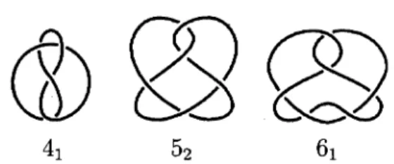
(4) 111. Volume Conjecture. For a knot. (1). K. in S^{3},. \displaystyle \lim_{r\rightar ow\infty}\frac{2 $\pi$}{r}\log|V_{K}^{(r)}($\xi$_{r})|=v_{3}|S^{3}\backslash K||,. where ||M|| is Gromov’s simplicial volume of a 3 manifold M and v3 is the hyperbolic volume of the regular ideal tetrahedron in the hyperbolic 3 space. If M is a hyperbolic manifold, then v_{3}||M|| is equal to the hyperbolic volume of M.. 4_{1} 5_{2} 6_{1}. FIGURE 2. The three simplest knots 4_{1}, 5_{2} and 6_{1} Kashaev checked such relation for the three simplest hyperbolic knots 4_{1}, 5_{2} and 6_{1} as follows. The invariants of these knots are. V_{4_{1} ^{(r)}($\xi$_{r})=\displaystyle \sum_{j=0}^{r-1}|($\xi$_{r})_{j}|^{2}, (x)_{j}=\prod_{k=1}^{j}(1-x^{k}) V_{5_{2}^{(r)}($\xi$_{r})=\displaystyle\sum_{0\leqj\leqk\leqr-1}\frac{$\xi$_{r}^{-j(+1)/2}($\xi$_{r})_{k}^{2}{($\xi$_{r}^{-1})_{k}, V_{6_{1}^{(r)}($\xi$_{r})=\displaystyle\sum_{0\leqj+k\leql\eqr-1}\frac{$\xi$_{r}^{(l-k1)(l-k+1)/2}|($\xi$_{r})_{l}|^{2}{($\xi$_{r})_{j}($\xi$_{r}^{-1})_{k},. ,. and numerical computation shows that. \displaystyle \lim_{\mathrm{r}\rightar ow\infty}\frac{2 $\pi$}{r}\log|V_{K}^{(r)}($\xi$_{r})|=2.0298 321\ldots \displaystyle \lim_{r\rightar ow\infty}\frac{2 $\pi$}{r}\log|V_{K}^{(r)}($\xi$_{r})|=2.82812208\ldots \displaystyle \lim_{r\rightar ow\infty}\frac{2 $\pi$}{r}\log|V_{K}^{(r)}($\xi$_{r})|=3.16396322\ldots. ,. ,. .. The righthand side numbers coincide with the hyperbolic volumes of the complements of these knots. For the figure‐eight knot 4_{1} , the above equality is actually proved by using the standard calculus. For other knots, to prove this conjecture is not so easy, but it is proved for some. simple hypergolic knots in [14] and [16]..
(5) 112. The colored Jones invariant V_{K}^{(r)}($\xi$_{r}) is a complex number and it is natural to consider about the meaning of the imaginary part or the argument. On the other hand, in the study of the hyperbolic volume, it turned out that the Chern‐Simons invariant must be the imaginary part of the hyperbolic volume, and now we call \mathrm{V}\mathrm{o}\mathrm{l}(M)+i\mathrm{C}\mathrm{S}(M) the complex volume of a hyperbolic manifold M . Actually, if we don’t take. the modulus in (1), we get the following conjecture which is proposed in [13]. Complexified Volume Conjecture. For a hyperbolic knot K,. \displaystyle \lim_{r\rightar ow\infty}\frac{2 $\pi$}{r}\log V_{K}^{(r)}($\xi$_{r})=\mathrm{V}\mathrm{o}\mathrm{l}(S^{3}\backslash K)+i. CS (S^{3}\backslash K). Here we are interested in the growth rate of imaginary part of the limit means. (\mathrm{m}\mathrm{o}\mathrm{d} i$\pi$^{2}\mathrm{Z}) .. V_{K}^{(r)}($\xi$_{r}). and so the. \displayst le\lim_{r\ightarow\infty}2$\pi$\arg\frac{V_{K}^{(r+1)}($\xi$_{r+1}){V_{K}^{(r)}($\xi$_{r}). 3. CHEN YANG ’ \mathrm{S} OBSERVATION -. The colored Jones invariants of knots and links are extended to the. Witten‐Reshetikhin‐Turaev invariant of 3 manifolds. But, for a 3 man‐ ifold M , we have. \displaystyle \lim_{r\rightar ow\infty}\frac{2 $\pi$}{r}\log$\tau$^{(r)}(M)=0. and the analogy of the volume conjecture for knots and links does not hold for the’ Witten‐Reshetikhin‐Turaev invariant. However, Q. Chen. and T. Yang found in [2] that the analogy of the volume conjecture. seems to hold for $\tau$^{(r)}(M) if r is odd and the parameter q is replaced by the second r‐th root of unity $\xi$_{r}^{2} instead of the first r‐th root of unity. $\xi$_{r}=\exp(2 $\pi$ i/r). .. Chen‐Yang’s Conjecture. Let. M. be a 3 manifold. Then. \displaystyle \lim_{n\rightar ow\infty}\frac{4 $\pi$}{2n+1}\log$\tau$^{(2n+1)}(M)|_{$\xi$_{2r $\iota$+1}\rightar ow$\xi$_{2n+1}^{2} =\mathrm{V}\mathrm{o}\mathrm{l}(M)+i CS(M). (\mathrm{m}\mathrm{o}\mathrm{d} i$\pi$^{2}\mathrm{Z}). .. They numerically checked the above for 3 manifolds obtained by some integral surgeries along the knots 4_{1} and 5_{2} . T. Ohtsuki an‐. nounced in [15] a proof for this conjecture for 3 manifolds obtained from the integral surgeries along 4_{1}..
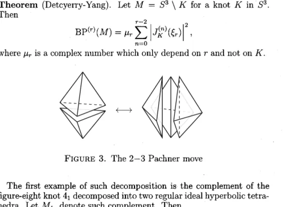
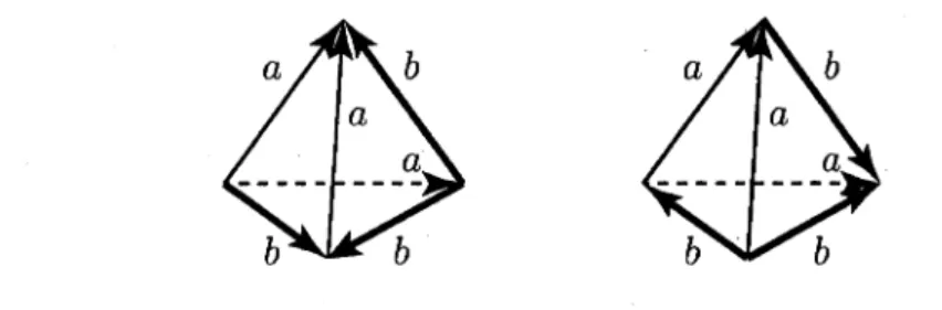
(6) 113. Chen and Yang also investigated the Turaev‐Viro invariant [22],. which is defined by using a tetrahedral decomposition of a 3 mani‐ fold. For a closed 3 manifold M , let \mathrm{T}\mathrm{V}^{(r)}(M) be the Turaev‐Viro. invariant of. M.. Then, it is known by [19] that. \mathrm{T}\mathrm{V}^{(r)}(M)=|$\tau$^{(r)}(M)|^{2} This relation is proved for the case q=$\xi$_{r} , but the proof works well for the case q=$\xi$_{r}^{2} if r is odd since $\xi$_{r}^{2} is also a primitive r‐th root of unity. Then Chen‐Yang’s conjecture implies that. \displaystyle \lim_{n\rightar ow\infty}\frac{2 $\pi$}{2n+1}\log|\mathrm{T}\mathrm{V}^{(2n+1)}(M)|_{$\xi$_{2n+1}\rightar ow$\xi$_{2n+1}^{2} =\mathrm{V}\mathrm{o}\mathrm{l}(M). .. The Turaev‐Viro invariant is generalized by Benedetti and Petronio. [1] to a 3 manifold. M. with cusp boundary or totally geodesic bound‐. ary decomposed into ideal tetrahedra or truncated tetrahedra which. is based on the Pachner move [18] generalized for such decomposition by J. Roberts. We denote this invariant by. Yang pointed out the following in [23]. Theorem (Detcyerry‐Yang). Let. Then. where. $\mu$_{r}. M. =. \mathrm{B}\mathrm{P}^{(r)}(M) .. Detcyerry and. S^{3}\backslash K for a knot. \displaystyle\mathrm{B}\mathrm{P}^{(r)}(M)=$\mu$_{r}\sum_{n=0}^{r-2}|J_{K}^{(n)}($\xi$_{r})|^{2},. is a complex number which only depend on. r. K. in S^{3}.. and not on. K.. \leftrightarrow. FIGURE 3. The 2‐3 Pachner move. The first example of such decomposition is the complement of the figure‐eight knot 4_{1} decomposed into two regular ideal hyperbolic tetra‐ hedra. Let M_{4_{1}} denote such complement. Then. \displaystyle \mathrm{B}\mathrm{P}^{(r)}(M_{4_{1} )=\sum_{a,b=0}^{(r-3)/2}d(2a+1)d(2b+1) \left\{ begin{ar y}{l } a&a&b\ b&b&a \end{ar y}\right\} left\{ begin{ar y}{l } a&a&b\ b&b&a \end{ar y}\right\}.
(7) 114. FIGURE 4. Decomposition of the figure‐eight knot complement The second example is the smallest hyperbolic 3 manifold with to‐. tally geodesic boundary M_{\min} , which is classified by Fujii [5]. This. manifold is obtained by two truncated regular tetrahedra whose dihe‐ dral angles are all equal to $\pi$/6 . All edges are glued to one edge and \mathrm{B}\mathrm{P}^{(r)}(M_{\min}) is given by. \displaystyle\mathrm{B}\mathrm{P}^{(r)}(M_{\min})=\sum_{a=0}^{(r-3)/2}d(2a+1)(\left\{ begin{ar ay}{l } a&a&a\ a&a&a \end{ar ay}\right\})^{2}. For Benedetti‐Petronio invariant, Chen and Yang observed its re‐ lation to the complex volume, and propose the following conjecture.. Volume Conjecture for Benedetti‐Petronio invariant (Chen‐ Yang). Let M be a hyperbolic manifold with cusp or totally geodesic boundary and. r. be an odd positive integer, then. \displaystyle \lim_{n\rightar ow\infty}\frac{2 $\pi$}{2n+1}\log \mathrm{B}\mathrm{P}^{(2n+1)}(M)|_{$\xi$_{2n+1}\rightar ow$\xi$_{2r $\iota$+1}^{2} =\mathrm{V}\mathrm{o}\mathrm{l}(M)+i CS(M). (\mathrm{m}\mathrm{o}\mathrm{d} i$\pi$^{2}\mathrm{Z}). 4. VARIOUS CONJECTURES. Chen‐Yang’s conjecture is generalized to various quantum SO(3) in‐. variants.. 4.1.. SO(3) ‐version. of the Witten‐Reshetikhin‐Turaev invari‐. ant. Let be a closed oriented three manifold. For a positive odd r integer greater than or equal to 3, let be the SO(3) ‐version M. $\tau$_{SO(3)}^{(r)}(M). of the Witten‐Reshetikhin‐Turaev invariant of M introduced in [8], and let be its modified SO(3) ‐version. Then \overline{ $\tau$}_{SO(3)}^{(r)}(M) =. $\tau$_{SO(3)}^{(r)}(M)|_{$\xi$_{r}\rightar ow$\xi$_{r}^{2}. the following may holds..
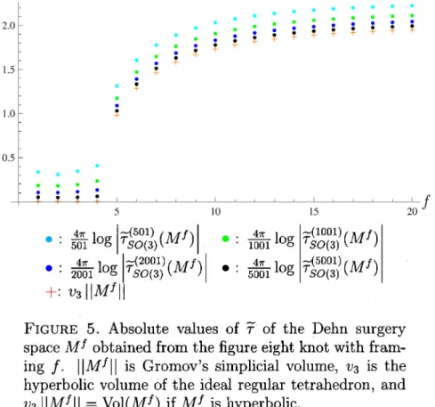
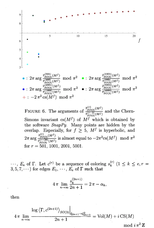
(8) 115. Conjecture 1 ( SO(3) ‐version of Chen‐Yang’s conjecture). Let. M. a closed oriented hyperbolic three manifold. Then. 4. $\pi$\displaystyle\lim_{n\rightar ow\infty}\frac{\log\overline{$\tau$}_{SO(3)}^{(2n+1)}(M)}{2n+1}=\mathrm{V}\mathrm{o}\mathrm{l}(M)+i. CS (M) .. be. (\mathrm{m}\mathrm{o}\mathrm{d} i$\pi$^{2}\mathrm{Z}) .. Now we compute the modified Witten‐Reshetikhin‐Turaev invariant of a three manifolds M^{f} which is obtained from the Dehn surgery of the figure eight knot K with framing f . We use the following notations.. \{n\}=$\xi$_{r}^{n}-$\xi$_{r}^{-n}, \{n, k\}=\{n\}\{n-1\}\cdots\{n-k+1\}, \{n\}!=\{n, n\}. Then the invariant. \overline{ $\tau$}_{SO(3)}^{(r)}(M^{f}) is given as follows.. \triangleleft_{$\tau$_{SO(3)}^{r)}(M^{f})=\sum_{n=0}^{(r-3)/2}q^{n^{2}+n}V_{n}^{(r)}(K)}\{2n+1\}\{1\} =\displaystyle \sum_{n=0}^{(r-3)/2}q^{n^{2}+n}\{2n+1\}\{1\} \sum_{k=0}^{2j}\frac{\{2n+1+k,2k+1\} {\{1\} .. (2). By using this formula, values of. \displaystyle \frac{4 $\pi$}{r}\log|\overline{ $\tau$}_{SO(3)}^{(r)}(M^{f})|. are given by the. graph in Figure 5. The Chern‐Simons part of the conjecture is checked. by computing the values. 2$\pi$\displaystle\arg\frac{\tilde{$\tau$}_{SO(3)}^{(r)}M^{f}) \tilde{$\tau$}_{SO(3)}^{(r-2)}(M^{f}). \mathrm{m}\mathrm{o}\mathrm{d} $\pi$^{2} , which are given by. the graph in Figure 6. The signature of the Chern‐SImons invariant is ambiguous because the the relation of the orientation of the manifold and the choice of q or q^{-1} is not fixed commonly, and here the signa‐ ture of CS and cs are opposite. The argument of such ratio seems to. estimate the Chern‐Simons invariant well for hyperbolic manifolds (Cf. computation in [13] also estimate the Chern‐Simons invariant well for knots). 4.2. Turaev‐Viro invariant. Let M be a closed oriented 3‐manifold and be the SO(3) ‐version of the Turaev‐Viro invariant. \mathrm{T}\mathrm{V}_{\mathcal{S}O(3)}^{(r)}(M). in [22] given by the quantum 6j symbol in the last section.. -(r). \mathrm{T}\mathrm{V}_{SO(3)}(M). Let. be the modified invariant which is obtained by replac‐. ing $\xi$_{r} by $\xi$_{r}^{2} . Then, from the relation Conjecture 1, we have. |^{\triangleleft_{$\tau$_{SO(3)}^{r)}(M)} |^{2}=\overline{\mathrm{T}\mathrm{V} _{SO(3)}^{(r)}(M) and. Conjecture 2. For a hyperbolic closed oriented three manifold M,. 2 $\pi$\displayst le\lim_{n\rightarow\infty}\frac{\log|\overline{\mathrm{T}\mathrm{V}_{SO(3)}^{(2n+1)}(M)|}{2n+1}=\mathrm{V}\mathrm{o}\mathrm{l}(M). ..
(9) 116. \bullet. :. \bullet. :. \displaystyle \frac{4 $\pi$}{501}\log|\overline{ $\tau$}_{SO(3)}^{(501)}(M^{f})| \displaystyle \frac{4 $\pi$}{20 1}\log $\tau$_{SO(3)}^{20 1)}\dashv(M^{f})| \bul et:\bul et. + : V3. :. ||M^{f}|. \displayte\frac{4$pi}501\logfrac{4$\pi}10 \logeft|bgin{ary}l \overin{$\tau}_{SO(3)^\mathr{l}0\mathr{l})(M^f\ dashv_{$\tu SO(3)}^{50\mathr{l})(M^f \end{ary}\ight|. FIGURE 5. Absolute values of 7 of the Dehn surgery space M^{f} obtained from the figure eight knot with fram‐ ing f. ||M^{f}|| is Gromov’s simplicial volume, v3 is the hyperbolic volume of the ideal regular tetrahedron, and v_{3}||M^{f}| =\mathrm{V}\mathrm{o}\mathrm{l}(M^{f}) if M^{f} is hyperbolic. Please note that the Turaev‐VIro invariant is a real number, and here we take the absolute value of it.. 4.3. Kirillov‐Reshetikhin invariant. Kirillov and Reshetikhin ex‐. tended the colored Jones invariant to knotted graphs with trivalent. vertices in [9]. This is also constructed by using the Kauffman bracket and Jones‐Wenzl idempotent in [7], which is called the quantum spin network. Here we consider the unitary version of the quantum spin. network in [3]. Let. $\Gamma$. \ldots,. \cdots,. be a trivalent knotted graph with edges E_{1}, E_{2}, j_{e} be an SO(3) ‐admissible coloring for corre‐ sponding edges of $\Gamma$ , and we denote the coloring by c. SO(3) ‐admissible E_{e} . Let j_{1}, j_{2},. means that each j_{k} is a positive odd integer and, for the three colors a, b, c of edges around a vertex, a+b+c is an odd integer and they satisfy the triangle inequalities 0 < a < b+c, 0 < b < c+a and 0<c<a+b . Let \{ $\Gamma$, c\rangle_{SO(3)} denote the SO(3) version of the unitary. spin network in [4], which is an invariant of knotted graphs. For this invariant, following may holds.. Conjecture 3. Let M\mathrm{b}\mathrm{e}_{\wedge} a hyperbolic cone manifold obtained from a knotted graph $\Gamma$ in S^{3} with the cone angles $\alpha$_{1}, \cdots, $\alpha$_{e} at edges E_{1},.
(10) 117. f. \bullet. :. \bullet. :. +. :. 2$\pi$\displaystle\arg\fac{\overline{$\tau$}_{SO(3)}^{(501)}(M^{f}) \overline{$\tau$}_{SO(3)}^{(49 )}(M^{f}) 2$\pi$\displaystle\arg\fac{\overline{$\tau$}_{SO(3)}^{(20(M^{f}) 1)}(M^{f}) \tilde{$\tau$}_{SO(3)}^{(19 )}(Mf)} -2$\pi$^{2}. \mathrm{m}\mathrm{o}\mathrm{d} $\pi$^{2}. \bullet. :. \mathrm{m}\mathrm{o}\mathrm{d} $\pi$^{2}. \bullet. :. \mathrm{m}\mathrm{o}\mathrm{d} $\pi$^{2}. cs. FIGURE 6. The arguments of. 22$\$pi\dpsila$yt\ea\arrggf_{c{\\tioldev$erauli}n_{SeO({3)\^o10ve)}(rMl^i{fne\o{ver$lin\{$t\atauu$}_{s}o_(3{)^S5O01(}3\ov)e}rl^in{{\$\ltaaun}_g{SOl(e3^499)}\_9{(M)^}(f})M{(M)^}f})f. \displaytle\frac{\tilde{$\tau$}_{SO(3)}^{r(M^{f})\tilde{$\tau$}_{SO(3)}^{r-2)}(MJ. \mathrm{m}\mathrm{o}\mathrm{d} $\pi$^{2}. \mathrm{m}\mathrm{o}\mathrm{d} $\pi$^{2}. and the Chern‐. Simons invariant \mathrm{c}\mathrm{s}(M^{f}) of M^{f} which is obtained by the software SnapPy. Many points are hidden by the overlap. Especially, for f \geq 5, M^{f} is hyperbolic, and. 2$\pi$\displaystle\arg\frac{\tilde{$\tau$}_{SO\langle3)}^{(r)}M^{f}) \overline{$\tau$}_{SO(3)}^{(r-29)}(Mf)}. for. r=501 ,. is almost equal to. -2$\pi$^{2}\mathrm{c}\mathrm{s}(M^{f}). 1001, 2001, 5001.. E_{e} of $\Gamma$ . Let c^{(r)} be a sequence of coloring 5, 7, ) for edges E_{1}, \cdots, E_{e} of $\Gamma$ such that. \ldots,. 3,. \mathrm{m}\mathrm{o}\mathrm{d} $\pi$^{2}. s_{k}^{(r)}. (1 \leq. k \leq e,. r. 4 $\pi$\displaystyle \lim_{n\rightar ow\infty}\frac{s_{k}^{(2n+1)} {2n+1}=2 $\pi-\alpha$_{k}, then. 4. $\pi$\displayst le\lim_{n\rightarow\infty}\frac{\log\langle$\Gam a$,c^{(2n+1)}\rangle_{SO(3)}1_{$\xi$_{2n+1}\rightarow$\xi$_{2n+1}^{2} {2n+1}=\mathrm{V}\mathrm{o}\mathrm{l}(M)+i. CS(M) \mathrm{m}\mathrm{o}\mathrm{d} i$\pi$^{2}\mathrm{Z}. =.
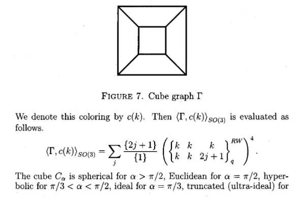
(11) 118. where. \langle $\Gam a$, c^{(2n+1)}\rangle_{SO(3)}. is the. SO(3). version of the Kirillov‐Reshetikhin. invariant, which is a restriction of the original Kirillov‐Reshetikhin in‐ variant to odd colors, and \mathrm{V}\mathrm{o}\mathrm{l}(M) and \mathrm{C}\mathrm{S}(M) are the hyperbolic vol‐ ume and the Chern‐Simons invariant of M_{$\alpha$_{1} $\alpha$_{l} respectively as before.. As a special case of this conjecture, we also have a conjecture for hyperbolic polyhedra. Conjecture 3’. Let P be a hyperbolic polyhedron with edges E_{1}, \cdots, E_{e} whose dihedral angles at E_{1}, \cdots, E_{e} are $\alpha$_{1}, \cdots, $\alpha$_{e} , and $\Gamma$ be the planar graph obtained by the edges of $\Gamma$ . Let c^{(r)} be a sequence of coloring s_{k}^{(r)} (1\leq k\leq e, r=3,5,7, \cdots) for edges E_{1}, \cdots, E_{e} of $\Gamma$ such that. 2 $\pi$\displaystyle \lim_{n\rightar ow\infty}\frac{s_{k}^{(2n+1)} {2n+1}= $\pi-\alpha$_{k} , then. 2 $\pi$\displayst le\lim_{n\rightarow\infty}\frac{\log\langle$\Gam a$,c^{(r)}\rangle_{SO(3)}1_{$\xi$_{2n+1}\rightarow$\xi$_{2n+1}^{2} {2n+1}=\mathrm{V}\mathrm{o}\mathrm{l}(P). .. This conjecture comes from Conjecture 3 since the corresponding cone. manifold is the double of P.. Now let us compare the volume of the regular hyperbolic cube C_{ $\alpha$} with dihedral angle $\alpha$ and the Kirillov‐Reshetikhin invariant of the graph $\Gamma$ formed by the edges of a cube whose edges are all colored by the same spin k . For the admissible condition, k must be an odd integer.. FIGURE 7. Cube graph. $\Gamma$. We denote this coloring by c(k) . Then \langle $\Gamma$, c(k)\rangle_{SO(3)} is evaluated as. follows.. \displaystyle\{$\Gam a$,c(k)\rangle_{\mathcal{S}O(3)}=\sum_{j}\frac{\2j+1\}{\1\} (\left\{ begin{ar ay}{l } k&k& &k\ k&k&2j&+1 \end{ar ay}\right\})^{4}. The cube C_{ $\alpha$} is spherical for $\alpha$> $\pi$/2 , Euclidean for $\alpha$= $\pi$/2 , hyper‐. bolic for $\pi$/3< $\alpha$< $\pi$/2 , ideal for $\alpha$= $\pi$/3 , truncated (ultra‐ideal) for.
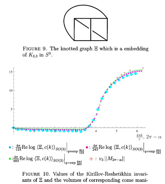
(12) 119. \overline{r} ’. 7 $\Gamma$- $\alpha$. c(k)\displaystyle \rangle_{SO(3)}|_{q=\exp\frac{4 $\pi$ i}{103} \bul et:\frac{2 $\pi$}{303}{\rm Re}\log( $\Gamma$, c(k)\rangle_{SO(3)}|_{q=\exp\frac{4 $\pi$ i}{303} \mathrm{V}\mathrm{o}\mathrm{l}(C_{ $\pi$- $\alpha$}) \displaystyle \bul et:\frac{2 $\pi$}{1003}{\rm Re}\log\{ $\Gamma$, c(k)\rangle_{SO(3)}|_{q=\exp\frac{4 $\pi$ i}{10 3} \displaystyle \bul et:\frac{2}{1}\mathrm{t}^{ \rm Re}\log}\langle $\Gamma$,. ---. :. FIGURE 8. Values of the Kirillov‐Reshetikhin invariants. of cubic graphs and the volumes of C_{ $\alpha$}.. 0\leq $\alpha$\leq $\pi$/3 and it becomes the right‐angled ideal regular cuboctahe‐. dron for $\alpha$=0 whose volume is 12.046. \cdots. .. Now we show the second example. Let K_{3,3} be the complete bipar‐ tite graph with six vertices and : be the knotted graph which is the embedding of K_{3,3} as in Figure 9. We give the coloring k for all edges and denote this coloring by c(k) . Then c(k)\rangle_{SO(3)} is given by. c(k)\rangle_{SO(3)}=. \displaystyle\sum_{j}(-1)^{k}q^{(k^{2}+k-j^{2}-j)/2}\frac{\ 2j+1\} {\ 1\} (\left\{ begin{ar ay}{l } k&k& &k\ k&k&2j&+\mathrm{l} \end{ar ay}\right\})^{3}. Some values of | c(k)\rangle_{SO(3)}| and some volumes of the corresponding cone manifolds are given in Figure 10. The arguments of c(k)\}_{SO(3)} are investigated in Figure 11. The author don’t know the definition of the Chern‐Simons invariant of the corresponding cone manifold and relation to the Chern‐Simons invariant is not checked yet. 4.4. Yokota invariant. The Kirillov‐Reshetikhin invariant is defined. for spatial graphs with trivalent vertices, while the Yokota invariant in. [24] is defined for spatial graphs with multivalent vertices. Let $\Gamma$. $\Gamma$. be. a colored spatial graph with odd colors and be a vertex of whose valency is k . We expand the vertex v as in Figure 12, and let \overline{$\Gam a$} be the v.
(13) 120. aph: which is a embedding. \overline{r} ’. \displaystyle \bul et:\frac{4 $\pi$}{123}{\rm Re}\log \displaystyle \bul et:\frac{4 $\pi$}{483}{\rm Re}\log. 2 $\pi$- $\alpha$. c(k)\rangle_{SO(3)}|_{q=\exp\frac{4 $\pi$ i}{123} \displaystyle\bulet:\frac{4$\pi$}{243}{\rmRe}\log c(k)\rangle_{\mathcal{S}O(3)}|_{q=\exp\frac{4 $\pi$ i}{243} | M_{2 $\pi$- $\alpha$}|| c(k)\rangle_{SO(3)}|_{q=\exp\frac{4 $\pi$ i}{483} + : V3. FIGURE 10. Values of the Kirillov‐Reshetikhin invari‐. ants of : and the volumes of corresponding come mani‐ fold M_{ $\alpha$} with the cone angle $\alpha$ for all edges where $\alpha$=0, $\pi$/5, 2 $\pi$/7, $\pi$/3, 2 $\pi$/5, $\pi$/2, 2 $\pi$/3 , which are computed by. the software Orb [17].. resulting graph. Now we define the Yokota invariant \langle\{ $\Gamma$, c\}\rangle_{SO(3)} by using the Kirillov‐Reshetikhin invariant. Here c denote the coloring of $\Gamma$.. \langle\langle $\Gamma$,. c\displaystyle\rangle\}_{SO(3)}=\sum_{i_{1},i_{p} \prod_{r=1}^{p}\frac{\ 2i_{r}+1\} {\ 1\} <\overline{$\Gam a$}, \tilde{C}>s. \tilde{c}>so(3). =$\Gam a$ is the mirror image of \overline{$\Gam a$} and \tilde{c} is the coloring of \overline{$\Gam a$} which is a extension of c by adding the coloring i_{1},. \cdots,. i_{p} for the newly added edges by the.
(14) 121. 1. \displayst le\frac{4$\pi$k}{r +. \bullet. :. :. \displaystle\frac{2$\pi$}{123}{\rmI }\log\frac{\langle-,c(k)\rangle_{SO(3)}|_{q=$\xi$_{123}^{2} \langle-,c(k)\rangle_{\mathcal{S}O(3)}|_{q=$\xi$_{125}^{2} \displaystle\frac{2$\pi}{243}{\rmRe}\logfrac{\lange^{\underline{=},\mathrm{c}(k)\}_{SO(3)}|_{\mathrm{q}=$\xi_{243}^{2 }(-,ck)\}_{SO(3)}|_{\mathrm{q}=$\xi_{245}^{2 } \displaystle\frac{2$\pi}{483}{\rmI }\logfrac{\lnge^{\underlin{=},\mathrm{c}(k)\rangle_{SO(3)}|_{\mathrm{q}=$\xi_{483}^{2}\lange-,\mathrm{c}(k)\_{SO(3)}|_{q=$\xi_{485}^{2} \bullet. :. FIGURE 11. Arguments of the Kirillov‐Reshetikhin in‐ variants of :. i_{1}. c. i_{2}. i_{3}. .. .. .. i_{k-3} k. \rightarrow c. \mathcal{C}_{2}. C_{3}. c_{4}. c_{k-1}. \overline{$\Gam a$}. $\Gamma$. FIGURE 12. Expansion at k‐valent vertex expansion of the multivalent vertices. This does not depend on the expansion of the multivalent vertices and this is actually an invariant of the spatial graph. For this invariant, following may holds.. Conjecture 4. Let M be a hyperbolic cone manifold obtained from a knotted graph $\Gamma$ in S^{3} with the cone angles $\alpha$_{1} , ) $\alpha$_{e} at edges E_{1}, \ldots, E_{e} of $\Gamma$ . Let c^{(r)} be a sequence of coloring s_{k}^{(r)} (1 \leq k \leq e, r =. 3,. 5, 7,. ) for edges E_{1},. \cdots,. E_{e} of $\Gamma$ such that 4. $\pi$\displaystyle \lim_{n\rightar ow\infty}\frac{s_{k}^{(2n+1)} {2n+1}. =.
(15) 122. 2. $\pi-\alpha$_{k} ,. then. 2 $\pi$\displaystyle\lim_{n\rightar ow\infty}\frac{\log\{ langle$\Gam a$',c^{(2n+1)}\ rangle_{SO(3)}|_{$\xi$_{2n+1}\rightar ow$\xi$_{2n+1}^{2} {2n+1}=\mathrm{V}\mathrm{o}\mathrm{l}(M). .. Conjecture 4’. Let P be a hyperbolic polyhedron with edges E_{1}, , E_{e} whose dihedral angles at E_{1}, \cdots, E_{e} are $\alpha$_{1}, \cdots, $\alpha$_{e} , and $\Gamma$ be the planar graph obtained by the edges of $\Gamma$ . Let c^{(r)} be a sequence of coloring s_{k}^{(r)} (1\leq k\leq e, r=3,5,7, \cdots) for edges E_{1}, \cdots, E_{e} of $\Gamma$ such \cdots. that. 2 $\pi$\displaystyle \lim_{n\rightar ow\infty}\frac{s_{k}^{(2n+1)} {2n+1}= $\pi-\alpha$_{k} , then. $\pi$\displaystyle\lim_{n\rightar ow\infty}\frac{\log\langle\langle$\Gam a$,c^{(2n+1)}\rangle\}_{SO(3)}|_{$\xi$_{2r$\iota$+1}\rightar ow$\xi$_{2n+1}^{2} {2n+1}=\mathrm{V}\mathrm{o}\mathrm{l}(P). .. For example, let $\Pi$ be a square pyramid with all dihedral angles $\alpha$ . If $\alpha$< $\pi$/2 , then $\Pi$ is realized as a truncated hyperbolic pyramid which is a half of the hyperbolic cube. The Yokota invariant of $\Pi$ with coloring c(k) which assigns a positive odd integer k to all edges is given by. \displaystyle\langle\langle$\Gam a$,c(k)\rangle\rangle_{SO(3)}=\sum_{j}\frac{\2j+1\}{\1\} (\left\{ begin{ar ay}{l } k&k& &k\ k&k&2j&+1 \end{ar ay}\right\})^{4}. This is equal to the Kirillov‐Reshetikhin invariant of the cube graph, and the Conjecture 4 seems to holds for this graph according to the computation in Figure 8. 5. CONCLUSION. By replacing the first primitive root of unity $\xi$_{r} =\exp(2 $\pi$ i/r) with the second primitive root of unity $\xi$_{r}^{2} , the volume conjecture for the quantum knot invariant is extended to various cases. I hope that the observations in this note will help to prove the conjecture generally. REFERENCES. [1] R. Benedetti and C. Petronio: On Roberts’ proof of the Turaev‐Walker theo‐ rem. J. Knot Theory Ramifications 5 (1996), 427‐439. [2] Q. Chen and T. Yang: A volume conjecture for a family of Turaev‐Viro type invariants of 3‐manifolds with boundary, preprint, arXiv:1503.02547.. [3J. $\Gamma$ .. Costantino, $\Gamma$ . Guéritaud and R. van der Veen: On the volume conjecture for polyhedra. Geom. Dedicata 179 (2015), 385‐409. [4] $\Gamma$ . Costantino and M. Murakami: On the SL(2, C) quantum 6j ‐symbols and their relation to the hyperbolic volume. Quantum Topol. 4 (2013), 303‐351. [5] M. Fujii: Hyperbolic 3‐manifolds with totally geodesic boundary which are decomposed into hyperbolic truncated tetrahedra. Tokyo J. Math. 13 (1990), 353‐373..
(16) 123 [6] R. M. Kashaev: The hyperbolic volume of knots from the quantum diloga‐ rithm. Lett. Math. Phys. 39 (1997), 269‐275. [7] L. H. Kauffman and S. L. Lins: Temperley‐Lieb recoupling theory and invari‐ ants of 3‐manifolds. Annals of Mathematics Studies, 134. Princeton University Press, Princeton, NJ, 1994.. [8] R. Kirby and P. Melvin: The 3‐manifold invariants of Witten and Reshetikhin‐ Turaev for sl(2, C) . Invent. Math. 105 (1991), 473‐545. [9] A. N. Kirillov and N. Yu. Reshetikhin, Representations of the algebra \mathcal{U}_{q}(sl(2)) , q ‐orthogonal. polynomials and invariants of links. Infinite‐dimensional Lie al‐. gebras and gròups (Luminy‐Marseille, 1988), 285‐339, Adv. Ser. Math. Phys., 7, World Sci. Publ., Teaneck, NJ, 1989.. [10] W. B. R. Lickorish:. The skein method for three‐manifold invariants. J. Knot Theory Ramifications 2 (1993), 171‐194.. [11] H. Murakami: Some limits of the colored Jones polynomials of the figure‐eight knot. Kyungpook Math. J. 44 (2004), 369‐383. [12] H. Murakami and J. Murakami: The colored Jones polynomials and the sim‐ plicial volume of a knot. Acta Math. 186 (2001), 85‐104. [13] H. Murakami, J. Murakami, M. Okamoto, T. Takata and Y. Yokota: Kashaev’s conjecture and the Chern‐Simons invariants of knots and links. Experiment.. Math. 11 (2002), 427‐435. [14] T. Ohtsuki: On the asymptotic expansion of the Kashaev invariant of the 5_{2} knot. to appear in Quantum Topology.. [15] T. Ohtsuki: A survey on the asymptotic expansion of the Kashaev invariant. of hyperbolic knots with up to 7 crossings, talk at Workshop on Volume Con‐ jecture and Quantum Topology, 2016 Sep. 6 to Sep. 9 at Waseda University.. [16] T. Ohtsuki and Y. Yokota:, On the asymptotic expansions of the Kashaev in‐. variant of the knots with 6 crossings, preprint, RIMS‐1865, www.kurims.kyoto‐. u. ac.jp/preprint/file/RIMS1865.pdf. [17] Home Page For Orb: http: / \mathrm{w}\mathrm{w}\mathrm{w} .ms.unimelb.edu.au /\sim \mathrm{s}\mathrm{n}\mathrm{a}\mathrm{p}/\mathrm{o}\mathrm{r}\mathrm{b} .html [18] U. Pachner: PL homeomorphic manifolds are ‐equivalent by elementary shelling, J. Combinatorics 12 (1991), 129‐145.. [19] J. Roberts: Skein theory and Turaev‐Viro invariants. Topology 34 (1995), 771‐ 787.. [20] N. Reshetikhin and V. G. Turaev: Ribbon graphs and their invariants derived from quantum groups. Comm. Math. Phys. 127 (1990), 1‐26. [21] N. Reshetikhin and V. G. Turaev: Invariants of 3‐manifolds via link polyno‐ mials and quantum groups. Invent. Math. 103 (1991), 547‐597. [22] V. G. Turaev and O. Ya. Viro: State sum invariants of 3‐manifolds and quan‐ tum 6j ‐symbols. Topology 31 (1992), 865‐902. [23] T. Yang: Volume Conjectures for Reshetikhin‐Turaev and Turaev‐Viro in‐ variants, talk at 2016 International Conference on Low‐dimensional Topology, Southwest Jiaotong University, Chengdu, China.. [24] Y. Yokota: Topological invariants of graphs in 3‐space. Topology 35 (1996), 77‐87.. DEPARTMENT OF MATHEMATICS, FACULTY OF SCIENCE AND ENGINEERING, WASEDA UNIVERSITY, OHKUBO, SHUNJUKU‐KU, TOKYO 169‐8555, JAPAN E‐mail address: [email protected].
(17)
図
+7


関連したドキュメント
Applying the representation theory of the supergroupGL(m | n) and the supergroup analogue of Schur-Weyl Duality it becomes straightforward to calculate the combinatorial effect
It leads to simple purely geometric criteria of boundary maximality which bear hyperbolic nature and allow us to identify the Poisson boundary with natural topological boundaries
As a consequence of this characterization, we get a characterization of the convex ideal hyperbolic polyhedra associated to a compact surface with genus greater than one (Corollary
Leibon’s construction is based on the idea of extending all the edges of the tetrahedron to infinity and dissecting the resulting polyhedron into 6 ideal tetrahedra and an
It is shown that the space of invariant trilinear forms on smooth representations of a semisimple Lie group is finite dimensional if the group is a product of hyperbolic
It is shown that the space of invariant trilinear forms on smooth representations of a semisimple Lie group is finite dimensional if the group is a product of hyperbolic
The theory of log-links and log-shells, both of which are closely related to the lo- cal units of number fields under consideration (Section 5, Section 12), together with the
We relate group-theoretic constructions (´ etale-like objects) and Frobenioid-theoretic constructions (Frobenius-like objects) by transforming them into mono-theta environments (and
