Comparison of clustering methods for single-cell transcriptome analysis

全文

(1)Vol.2017-BIO-51 No.2 2017/9/26. IPSJ SIG Technical Report. Comparison of clustering methods for single-cell transcriptome analysis YUJI KOZAKURA†1 TOMOYA MORI†1 WATARU FUJIBUCHI†1 Abstract: Single-cell transcriptome can provide information of global gene expression pattern in individual cells, so that detailed cell type classification considering cellular heterogeneity becomes more important to analyze complex biological system. Here we surveyed 12 clustering methods utilized for single-cell transcriptome analysis. We evaluated the performance of each method using published data of 1,830 single-cell transcriptome obtained from SHOGoiN database. Each single-cell transcriptome data was labeled by source tissues (adipose tissue, blood, brain, early embryonic tissue, genitalium, muscle, pancreas, skin). In the evaluation, we chose two criteria; normalized mutual information (NMI) and the purity. After optimizing the parameters by NMI, we calculated the sum of the NMI and the purity. As a result, the combination of the DBSCAN algorithm and t-SNE clustering showed the best performance on our data set. Keywords: clustering, single-cell, transcriptome, cell type classification, and gene expression analysis. 1. Introduction Recent single-cell transcrptome techniques provide new insights into cellular heterogeneity, which is important in various biological contexts, e.g. ontogeny, stress response, and physiology [1]. Therefore, detailed cell type classification is indispensable to undetstand complex biological system at a cell level. Currently, many dimensional reduction techniques and clustering methods are used for transcriptome analysis. For example, multivariate statistical technique, such as principal component analysis (PCA) [2], has often been used for transcriptome analysis since the early 2000s [3]. PCA is one of the linear methods, which perform a linear mapping of a high-dimensional input data to a low-dimensional space, helps us to extract important factors originating different cell types and to visualize the similarity between samples. Non-metric multidimensional scaling (NMDS) has also been used as a classical technique [4]. Non-linearity is taken into consideration in NMDS. Clustering methods classify the data points based on the result of dimensionality reduction. k-means [5] and DBSCAN [6, 7], for instance, are well known as classical clustering methods. In addition to the classical methods, recent techniques, such as t-distributed stochastic neighbor embedding (t-SNE) [8] and affinity propagation clustering (AP clustering) [9], are drawing attention in many fields including bioinformatics. t-SNE is a dimensionality reduction technique and has been used well because of its good performance [10]. AP clustering is also used for clustering of high-dimensional data with the characteristics of unbiased clustering. Besides these methods, rare cell type identification (RaceID) is specialized for identifying low population cell types [11]. A multi-kernel learning method, SIMLR, shows better performance for cell type classification than t-SNE and other classical methods under certain conditions [12].. In this paper, our aim is to gain insight and information into the variety of single-cell transcriptome clustering methods; we have evaluated the following twelve clustering methods from the viewpoint of single-cell classifications: 1. AP clustering 2. AP clustering on NMDS 3. DBSCAN on NMDS 4. k-means on NMDS 5. AP clustering on PCA 6. DBSCAN on PCA 7. k-means on PCA 8. RaceID 9. AP clustering on t-SNE 10. DBSCAN on t-SNE 11. k-measns on t-SNE 12. SIMLR We compared the performance of these methods using 1,830 human single-cell transcriptome data. These data can be obtained from the SHOGoiN (the Human Omics Database for the Generation of iPS and Normal Cells) database (http://shogoin.stemcellinformatics.org). Our evaluation of clustering methods also provides additional insights into clustering analysis of single-cell transcriptome data. The result indicates the importance of preprocessing step and the necessity of a framework or tools, which enable us to compare and evaluate the result of clustering by specific criteria.. 2. Methods First, we summarize recent clustering methods and dimensionality reduction techniques, and then describe the processing of data set and the criteria for evaluation of the performance used in this comparison.. †1 Center for iPS Cell Research and Application, Kyoto University. ⓒ2017 Information Processing Society of Japan. 1.

(2) Vol.2017-BIO-51 No.2 2017/9/26. IPSJ SIG Technical Report. 2.1 Affinity propagation clustering algorithm Affinity propagation clustering [9] is an unbiased clustering that runs without setting the number of final clusters. This method has been used in many fields, e.g. image analysis [13], the vehicle ad hoc networks [14] and gene expression analysis [15, 16, 17]. Affinity propagation algorithm takes a similarity c(i,j) between data point i and j as input. This algorithm supports negative Euclidean distance, or any other function for definition of similarity. Each data point i has a self-similarity, s(i,i), which influences the number of determined exemplars representing a cluster. The value of self-similarity is set by user. Initialized data points with a larger self-similarity are more likely to become exemplars. To determine clusters and exemplars, data points transmit two types of messages, responsibility and availability. The responsibility, r(i,j), is transmitted from data point i to candidate exemplar data point j and indicates how well suited data point j is as exemplar for data point i, The availability, a(i,j), is transmitted from candidate exemplar j to i responding to responsibility, which indicates that data point j is appropriate as exemplar for i based on supporting feedback from other data points. The self-responsibility, r(i,i) and self-availability, a(i,i) reflect the probability that data point i is suitable to an exemplar.. r(i, k) ← s(i, k) − max {a(i, k ') + s(i, k ')} , k 's.t.k '≠k. a(i, k) ← min{0, r(k, k) +. ∑. max{0, r(i', k)}},. i's.t.i'∉{i,k}. a(k, k) ←. ∑. max{0, r(i', k)}.. 2.3 t-Distributed Stochastic Neighbor Embedding (t-SNE) t-SNE [8] converts each data point from high-dimensional data into corresponding point in low-dimensional map where feature of the distance between each points in high dimension space is maintained. t-SNE has been used as a major visualization and clustering method for transcriptome analysis in recent years [10]. t-SNE algorithm calculates a similarity score in the original high-dimensional space. In t-SNE algorithm, the distance between high-dimensional data points is represented by conditional probability p j|i,. p j|i =. exp(− || xi − x j ||2 /2σ i2 ). ∑ exp(− || x − x i. j. ||2 /2σ i2 ). ,. k≠i. ||xi – xj|| is Euclidean distance between data point xi and xj. σ for each data point is chosen so that the perplexity of pj|i has a value close to the user defined perplexity. This value influences the number of nearest neighbors taken into account when building up the embedding in the low-dimensional space. The following assumption is introduced to reduce calculation cost,. pij =. p j|i + pi| j . 2n. For the low-dimensional space t-SNE use the t-distribution with one degree of freedom as the distribution of the distances to counterpart yi and yj to data point xi and xj in low-dimensional space,. i's.t.i'≠k. These messages are updated iteratively until the messages converge. When the summation of a point’s self-responsibility and self-availability becomes positive, that point becomes the exemplar. the exemplar of a data point i’s cluster is the data point j maximizing the following equation,. arg max{a(i, j) + r(i, j)}.. q j|i =. (1+ || yi − y j ||2 )−1. ∑(1+ || y − y i. j. ||2 )−1. .. k≠i. t-SNE performs dimensional reduction by minimizing the Kullback-Leibler divergence between these two distributions qij and pij.. j. 2.2 Rare cell type identification (RaceID) RaceID [11] is specialized for single-cell transcriptome analysis. This method was developed especially for rare cells. The first step of RaceID is gene selection which removes low expression genes and low quality samples. Then RaceID normalize processed data, and determines clusters by k-means clustering using the similarity in expression between samples based on Pearson correlation. The number of clusters is determined using the gap statistic. After the initial clustering step, RaceID detects outlier cells, which do not fit the model built up by considering technical and biological noise. The algorithm of this part has been used in the classification of rare cell populations.. ⓒ2017 Information Processing Society of Japan. 2.4 Single-cell interpretation via multi kernel learning (SIMLR) SIMLR [12] is a method utilizing multi-kernel learning for single-cell transcriptome. For single-cell transcriptome analysis, it is a problem that the diverse statistical characteristics of single-cell transcriptome can not be easily expressed by specific statistical model. Therefore, SIMIR used multiple kernels learning to learn similarity between data points by considering multiple statistical models. It takes gene expression information as an input matrix and learns a set of cell-to-cell similarities by estimating multiple kernels (Gaussian kernels), with taking the assumptions that C separable populations exist. The number of C is a parameter determined by the user. SIMLR makes the similarity matrix be confined to a C block-diagonal structure.. 2.

(3) Vol.2017-BIO-51 No.2 2017/9/26. IPSJ SIG Technical Report. Learned similarities can be used to visualize the cells, reduce the dimension of the data, and so on. 2.5 Data set selection Gene expression data of published 1,830 single-cell transcriptome were downloaded from SHOGoiN database (http://shogoin.stemcellinformatics.org) as of July 15, 2017 (adipose tissue: 44 samples, blood: 29 samples, brain: 475 samples, early embryonic tissue: 165 samples, genitalium: 331 samples, muscle: 316 samples, pancreas: 64 samples, and skin: 406 samples). 2.6 Input data sets. The number of the samples downloaded from SHOGoiN database was 1,830. Total mapped fragment counts in gene region were normalized as 1,000,000 per sample. Read counts were converted to log2 scale after adding 1 to avoid log of 0. Furthermore, some genes were removed, which were not transcribed in any sample. 59,239 genes were transcribed at least once in eight source tissue samples. The gene expression matrix was used as input for evaluation of clustering performance. 2.7 Sample label 1,830 samples were labeled by 8 different kinds of tissues. 2.8 Normalized Mutual Information (NMI) We chose NMI as a criterion for clustering evaluation. NMI indicates the consistency between the clustering result and the true labels of the n cells [19]. Given two clusters U and V on a set of data points, NMI is defined as: I(U,V)/max{H(U),H(V)}, where I(U,V) is the mutual information between U and V, and H(U) and H(V) represents the entropy of the clustering U and V. When U has P clusters, and V has Q clusters, the mutual information is calculated as the following equation, P. Q. I(U,V ) = ∑∑ p=1 q=1. |U p  Vq | N. log. N |U p  Vq | |U p | × | Vq |. ,. where |Up| and |Vq| indicates the cardinality of the p-th cluster in U and the q-th cluster in V respectively. The entropy of each cluster assignment is calculated by p. |U p | |U | log p , N p=1 N. H (U) = −∑ Q. | Vq | |V | log q . N q=1 N. H (V ) = −∑. NMI takes on values between 0 and 1, measuring the concordance of two clustering results. NMI is affected by the accuracy of clustering and subdivision of cluster. The value is 1 when the labels determined by the clustering result correspond with true labels. We calculated NMI using compare function in igraph library of R package. 2.9 Purity We also evaluated clustering results by a purity, which is an indicator to measure clustering performance. Label of largest. ⓒ2017 Information Processing Society of Japan. subset in each cluster is determined and then the total numbers of determined labeled samples are counted in each cluster. The summation of the total numbers is divided by the samples number N.. purity(U,V ) = −∑ P. max q |U p  Vq | . N. The purity is also a value between 0 and 1 and a higher purity indicates a better consistency between the labels determined by clustering and true labels. We calculated the purity obeying to above equation using standard cross table functions of R. 2.10 Optimal Eps (OptEps) of DBSCAN The optimal value of parameter Eps for DBSCAN was calculated obeying to reported method [20]. First, Euclidean distance was calculated on each pair of data point in two-dimensional space after dimensionality reduction. We used dist function of R to calculate distance between each point. Furthermore, the distance was converted into a matrix using as.matrix function and then three nearest neighbors of each data point were extracted. The number of data point pairs were plotted along the distance, and we choose the first slope change point in the plot as optimal eps value using R package changepoint. 2.11 Affinity propagation clustering We used apcluster function of R to determine the clusters in input data points by affinity propagation clustering algorithm. Optimal parameters were determined as produced highest NMI and highest sum of NMI and the purity by a grid search (The searching range of the parameters q and seeds are q = 0, 0.1, 0.2, 0.3, 0.4, 0.5, 0.6, 0.7, 0.8, 0.9, and 1.0 (default 0.5), and seed = 0, 100, 200, 300, 400, 500, 600, 700, 800, 900, and 1000). 2.12 NMDS combination clustering methods (NMDS + AP clustering, NMDS + DBSCAN, and NMDS + k-means) We used isoMDS function of R package MASS to convert high-dimensional data into a two-dimensional NMDS data. The dimensionality reduction data are clustered by affinity propagation algorithm. Optimal parameters were determined by the highest NMI and the highest sum of NMI and the purity using a grid search as explained in AP clustering section. The NMDS data were also clustered by DBSCAN method. We used dbscan function of R package dbscan. Optimal parameters were determined by the highest NMI and the highest sum of NMI and the purity (The searching range of the parameter eps are eps = OptEps −（OptEps/2）×0, OptEps – (OptEps/2) × 1, …, OptEps + (OptEps/2) × 8 with a fixed parameter minPts = 1). The NMDS data were also clustered by k-means method using kmeans function of R. The parameter determining the number of final clusters was set to 8. 2.13 PCA combination clustering methods (PCA + AP clustering, PCA + DBSCAN, and PCA + k-means) We used prcomp function of R package to convert high-dimensional data into a two-dimensional data defined by the principal component 1 and 2. The dimensionality reduction. 3.

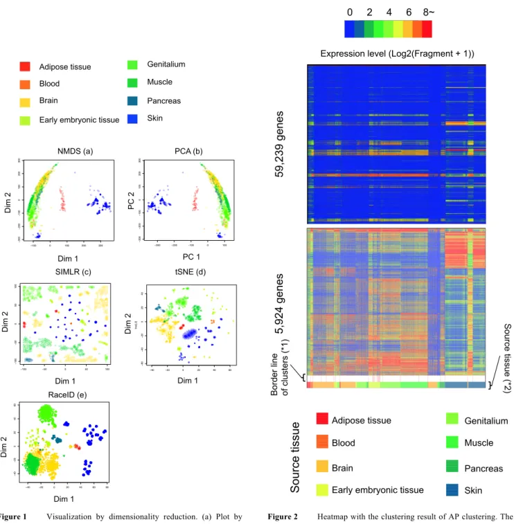
(4) Vol.2017-BIO-51 No.2 2017/9/26. IPSJ SIG Technical Report. data were clustered by affinity propagation algorithm. Optimal parameters were determined by the same method described in NMDS section. The PCA data were also clustered by DBSCAN method. Optimal parameters were determined by the same method described in NMDS section. The PCA data were also clustered by k-means method using kmeans function of R. The parameter determining the number of final clusters was set to 8. 2.14 RaceID We used R script for RaceID algorithm to calculate clusters in input data points, and the optimal parameters were determined by the highest NMI and the highest sum of NMI and the purity. The following are final parameters to choose: 1. A) B). Parameters of filterdata function Selected parameter: downsample = TRUE or FALSE Fixed parameters: mintotal = 3000 minexpr = 5, minnumber = 1, maxexpr = 500,dsn = 1, reseed = 17000 2. Parameters of clustexp function A) Selected parameter: do.gap = TRUE or sat = TURE, clustnr = 30 with cln = 0 or clustnr = 8 with cln = 8 B) Fixed parameters: bootnr = 50, metric = ”pearson”, SE.method = ”Tibs2001SEmax”, SE.factor = .25,B.gap = 50, rseed = 17000, FUNcluster = ”kmedioids”, clustnr = 30, cln = 0 3. Parameters of findoutliers function ouminc = 5, outlg = 2, probthr = 1e-3, thr=2**-(1:40), outdistquant = .95 4. Parameters of comtsne function rseed=15555, sammonmap = FALSE, initial_cmd = TRUE. R scripts was downloaded from https://github.com/dgrun/RaceID. 2.15 t-SNE combination clustering methods (t-SNE + AP clustering, t-SNE + DBSCAN, and t-SNE + k-means We used Rtsne function of R package Rtsne to convert high-dimensional data into a two-dimensional data. The t-SNE data were clustered by affinity propagation algorithm. Optimal parameters were determined by the same method described in AP clustering section. The searching range of parameter perplexity is perplexity = 5, 25, 50, …, 150, and the parameter pca was fixed with FALSE. The t-SNE data were also clustered by DBSCAN method. Optimal parameters were determined by the same method described in NMDS section. The t-SNE data were also clustered by k-means method using the same parameters in NMDS section. 2.16 SIMLR We used SIMLR function of R package SIMLR to determine the clusters in input data points and optimal parameters were determined by the highest NMI and the highest sum of NMI and the purity (The selected parameters : cores.ration= 0 or 1. The parameter c was set to 8 as the number of final clusters). ⓒ2017 Information Processing Society of Japan. 3. Results 3.1 The combination method of DBSCAN and t-SNE outperformed in separating eight source tissue derived cells 1,830 single-cell transcriptome data from SHOGoiN database labeled by source tissue types were utilized to evaluate twelve clustering methods. We evaluated the performance of the clustering by NMI and the purity. Lower NMI indicates low accuracy of clustering boundaries or excessive subdivisions of a cluster, and the purity indicates the label diversity level in each cluster. For each method, parameters with the highest score of NMI were chosen. In the case that multiple parameters result in the same NMI score, the parameter with higher purity was taken. The sum of NMI and the purity were used as final score for evaluation of clustering performance. Results showed that t-SNE + DBSCAN performed best among all the methods (NMI + purity = 1.65) (Table 1). Among the methods that require the pre-set cluster number, the combination method of t-SNE + k-means showed the best performance (NMI + purity = 1.55). 3.2 Visualization of the cells in featured space All the methods except AP clustering can visualize the feature of high-dimensional gene expression data as two-dimensional plots (Fig. 1). Although PCA and NMDS successfully clustered cells from adipocyte tissue and skin, they found difficulty in clustering cells from the other tissues (Fig. 1 a, b). On the other hand, RaceID, which is based on t-SNE at visualization, showed the better clustering compared with t-SNE to be influenced by the selection step of genes (Fig. 1 d, e) and the scatterplot indicated that RaceID has potential to separate eight source tissue cells. With regards to SIMLR, separation of cells from different source tissues was successful while the dispersion was larger than other methods (Fig. 1 c). For AP clustering, the results were only shown by heatmap (Fig. 2). It was noteworthy that AP clustering showed an advantage in subtypes clustering with high purity (0.89, Table 1).. 4. Discussion We compared twelve clustering methods. The results showed that t-SNE performed well in clustering large scale tissue types. It is reasonable result due to the recent popularity of t-SNE. As for AP clustering algorithm and RaceID in clustering large scale tissue types, AP clustering algorithm (the number of cluster = 28) and RaceID (the number of cluster = 41) might be underestimated (Table 1) because each source tissue may contain more cell types. Therefore, detailed investigations are necessary in the future. Besides, the t-SNE based plot of RaceID indicates that gene selection step should be important for appropriate clustering (Fig. 1). In the field of cell classifications, gene selection methods become more important to clearly separate various cell types at single-cell level. Gene selection and normalization of RaceID showed better performance for a large scale of data sets (Table 1, Fig. 1). However, the idea of selection by RaceID is not perfect, thus recent clustering methods at gene level [21][22] may be worth considering for. 4.

(5) Vol.2017-BIO-51 No.2 2017/9/26. IPSJ SIG Technical Report. further improvement. The multi-kernel learning of SIMLR also showed better performance in clustering a large scale of data sets (Table 1). The performance of any algorithm might be changed by requirement of setting parameters. Therefore, there is still room for improvement. Machine learning methods using the combination of multiple statistical models would become stronger in the future and accordingly prediction methods to approximate cluster numbers could be required based on biological feasibility. From our results, it is also indicated strongly that a framework or tools to compare the clustering results by specific criteria be required for sophisticated single-cell transcriptome analysis. Table 1. Clustering results of each method using optimal parameters. The first column shows clustering method and the second column indicates highest NMI when optimal parameters were searched. The third column indicates highest purity when optimal parameters were searched. The fourth column indicates the sum of NMI and the purity. The fifth column indicates the minimum number of clusters within parameter sets of same NMI and the purity. Asterisk indicates the method with setting parameter of final cluster number.. Method (Clustering methods). NMI. Purity. NMI + purity. AP clustering NMDS + AP clustering NMDS + DBSCAN NMDS + k-means * PCA + AP clustering PCA + DBSCAN PCA + k-means * RaceID SIMLR* t-SNE + AP clustering t-SNE + DBSCAN t-SNE + k-means *. 0.66 0.52 0.50 0.54 0.52 0.50 0.54 0.70 0.69 0.75 0.75 0.71. 0.89 0.72 0.50 0.72 0.72 0.50 0.71 0.88 0.80 0.88 0.90 0.84. 1.54 1.24 1.00 1.26 1.24 1.00 1.25 1.58 1.49 1.63 1.65 1.55. The number of clusters 28 10 7 8 10 7 8 41 8 10 10 8. References [1]Eldar, Avigdor, and Michael B. Elowitz. : Functional roles for noise in genetic circuits, Nature, Vol. 467, No.7312, pp. 167-173 (2010) [2]Hotelling, H. : Analysis of a complex of statistical variables into principal components, Journal of educational psychology, Vol.24, No.6, pp. 417-441 (1933) [3]Raychaudhuri, S., Stuart, J. M., & Altman, R. B. : Principal components analysis to summarize microarray experiments: application to sporulation time series, Pacific Symposium on Biocomputing, pp. 455-466, (2000) [4]Venerables, W. N., and B. D. Ripley. : Modern applied statistics with S, New York:Springer (2002) [5]Hartigan, John A., and Manchek A. Wong. : Algorithm AS 136: A k-means clustering algorithm, Journal of the Royal Statistical Society. Series C (Applied Statistics) Vol. 28, No.1, pp. 100-108 (1979). ⓒ2017 Information Processing Society of Japan. [6]Ester, M., Kriegel, H. P., Sander, J., & Xu, X. : A density-based algorithm for discovering clusters in large spatial databases with noise, Kdd. Vol. 96. No. 34. (1996) [7]Böhm, C., Kailing, K., Kröger, P., & Zimek, A. : Computing clusters of correlation connected objects, Proceedings of the 2004 ACM SIGMOD international conference on Management of data. ACM (2004) [8]Maaten, L. V. D., & Hinton, G. : Visualizing data using t-SNE, Journal of Machine Learning Research Vol.9. pp. 2579-2605 (2008) [9]Frey, B. J., & Dueck, D. : Clustering by passing messages between data points, science Vol.315, No.5814, pp.972-976 (2007) [10]Muraro, M. J., Dharmadhikari, G., Grün, D., Groen, N., Dielen, T., Jansen, E., ... & van Oudenaarden, A. : A single-cell transcriptome atlas of the human pancreas, Cell systems, Vol.3, No.4, 385-394 (2016) [11]Grün, D., Lyubimova, A., Kester, L., Wiebrands, K., Basak, O., Sasaki, N., ... & van Oudenaarden, A. : Single-cell messenger RNA sequencing reveals rare intestinal cell types, Nature, Vol.525, No.7568, pp.251-255 (2015). [12]Wang, B., Zhu, J., Pierson, E., Ramazzotti, D., & Batzoglou, S. : Visualization and analysis of single-cell RNA-seq data by kernel-based similarity learning, Nature Methods, Vol.14, No.4, pp.414-416 (2017) [13]Zhang, S., Zhan, Y., Dewan, M., Huang, J., Metaxas, D. N., & Zhou, X. S. : Deformable segmentation via sparse shape representation, In International Conference on Medical Image Computing and Computer-Assisted Intervention, Heidelberg. pp. 451-458 (2011) [14]Shea, C., Hassanabadi, B., & Valaee, S.. : Mobility-based clustering in VANETs using affinity propagation, Global telecommunications conference, IEEE. pp.1-6 (2009) [15]Joost, S., Zeisel, A., Jacob, T., Sun, X., La Manno, G., Lönnerberg, P., ... & Kasper, M. : Single-cell transcriptomics reveals that differentiation and spatial signatures shape epidermal and hair follicle heterogeneity, Cell systems, Vol.3, No.3, pp. 221-237 (2016) [16]Garnett, M. J., Edelman, E. J., Heidorn, S. J., Greenman, C. D., Dastur, A., Lau, K. W., ... & Liu, Q. : Systematic identification of genomic markers of drug sensitivity in cancer cells, Nature, Vol.483, No.7391, pp.570-575 (2012) [17]Cadwell, C. R., Palasantza, A., Jiang, X., Berens, P., Deng, Q., Yilmaz, M., ... & Sandberg, R. : Electrophysiological, transcriptomic and morphologic profiling of single neurons using Patch-seq, Nature biotechnology, Vol.34, No.2, pp.199-203 (2016) [18]E. Hinton and S.T. Roweis. : Stochastic Neighbor Embedding, In Advances in Neural Information Processing Systems, Vol.15, pp.833-840 (2002) [19]Strehl, A., & Ghosh, J.. : Cluster ensembles---a knowledge reuse framework for combining multiple partitions, Journal of machine learning research, Vol.3, pp.583-617 (2002) [20]Rahmah, N., & Sitanggang, I. S. : Determination of optimal epsilon (eps) value on dbscan algorithm to clustering data on peatland hotspots in sumatra, IOP Conference Series: Earth and Environmental Science, Vol.31, No.1 (2016) [21]Kiselev, V. Y., Kirschner, K., Schaub, M. T., Andrews, T., Yiu, A., Chandra, T., ... & Hemberg, M. : SC3-consensus clustering of single-cell RNA-Seq data, Nature Methods, Vol.14, No.5, pp.483-486 (2017). [22]Langfelder, P., & Horvath, S. : WGCNA: an R package for weighted correlation network analysis, BMC bioinformatics, Vol.9, No.1 pp.559 (2008). Acknowledgments This work was supported by Center for iPS Cell Research and Application (CiRA).. 5.

(6) Vol.2017-BIO-51 No.2 2017/9/26. IPSJ SIG Technical Report. 0 2 4 6 8~"" 0""""""2""""""4""""""6"""""8. Genitalium. Blood. Muscle. Brain. Pancreas. Early embryonic tissue. Skin. 300 200 100. ●. ● ●. ● ● ● ● ●● ● ● ● ● ● ● ● ● ● ● ●● ● ● ● ●● ● ● ● ● ● ● ● ● ● ● ● ● ● ● ● ● ● ● ● ● ● ● ● ● ● ● ● ●● ●● ● ● ● ●● ●. ● ●● ● ● ● ● ● ● ●● ● ● ● ● ● ● ●● ● ● ● ● ● ● ● ● ● ● ● ● ● ●● ● ● ● ● ● ● ● ●● ● ● ● ● ●● ● ● ● ● ● ● ●● ● ● ● ● ● ● ● ● ● ● ● ● ● ● ● ● ● ● ● ● ●● ● ● ● ●● ●. −200. ● ● ●● ● ● ● ●● ● ● ● ● ● ● ● ●●● ● ● ● ● ● ● ● ● ●● ● ● ● ● ● ●● ●● ● ● ● ●● ● ● ●● ● ● ●●● ● ● ● ● ● ● ● ● ● ● ● ● ● ● ● ● ● ● ● ● ● ● ● ●● ● ●●● ● ● ●. ●. ● ● ● ● ● ●. 0. ● ●. PC2. ● ● ●. ● ● ● ● ● ● ● ● ● ● ● ●● ● ● ●● ● ● ● ● ● ● ● ●●● ●● ● ● ● ● ●● ● ●● ● ● ● ● ● ●● ● ● ● ●● ●● ●●● ● ● ● ●● ● ● ●●. ● ●●. ●●. ●. ●. PC 2. ●. 100. 200. −300. 300. −200. ●. ● ● ● ●● ● ● ● ● ● ● ● ●● ● ● ●. ●. −50. ● ● ● ● ● ●● ●. −100. ● ● ● ● ● ● ●. ●. ●. ● ● ● ● ● ● ● ● ● ● ● ●● ● ● ● ● ● ●. ●. ● ● ●● ●● ●● ●● ● ●● ● ●●● ● ●●●. ● ● ● ● ● ● ● ● ● ●● ● ●● ● ● ● ● ● ● ● ● ●● ● ● ● ● ● ●●●● ●● ●● ●● ● ●●● ● ● ● ● ● ●● ●●● ● ● ● ●●● ● ● ● ●● ● ● ● ●● ● ● ●●● ● ●●● ● ● ● ●● ●●●●●●● ●●●● ●●●●●●●● ●● ●● ●● ●● ●●●●● ●●●● ●● ●●● ●● ● ● ● ●● ● ● ● ● ● ● ●●● ● ● ●●●●● ●● ●● ● ● ● ● ● ● ●● ● ●●● ● ●● ●●●● ● ● ● ● ●●●● ●● ●●●●●● ●● ● ● ●●●● ● ● ●●●●● ● ● ●● ●● ● ●●● ● ● ● ● ●● ● ● ● ●● ●● ●●●● ●●● ●● ●● ●● ●●● ● ● ●● ●● ●● ●●●● ● ●●● ●● ●● ●● ●●●● ● ● ●● ● ●● ● ●●● ● ●● ● ● ●● ● ●● ●●●● ●● ●● ● ●●● ●● ● ● ● ● ●●●●●● ● ●● ●● ●●●●● ● ●● ●● ●● ●● ● ●●●● ●● ●●●●● ●●●●● ●●●●● ● ●● ●● ● ● ● ●● ● ●● ●● ● ● ●●●●●● ● ●● ● ● ●●● ● ● ● ● ● ● ● ● ● ● ● ●● ● ● ● ●● ●● ● ● ● ●● ● ●●●● ●● ●● ●●●● ●●● ● ● ● ●● ● ●● ● ● ● ●●● ● ●● ● ●● ● ●● ●●●● ● ●● ●● ●●●●● ● ●● ● ● ●● ● ● ● ● ● ●● ● ● ● ● ● ● ● ● ● ● ● ● ● ● ● ● ● ● ● ● ●●●● ● ●● ● ●● ● ●●● ● ● ●● ●● ● ● ● ● ● ●●● ● ● ●● ● ● ● ● ●●●●● ●●● ●● ● ●● ●● ●●●● ●●●●●●● ● ●● ● ●● ● ●● ● ● ● ● ●●● ●●● ●●●● ● ● ●● ● ●●● ● ● ●●●●●●●●●●●●●●●● ●●●● ●●. −100. −50. 0. 50. 100. 40. ● ● ● ● ● ● ● ● ● ● ● ● ● ● ● ● ●● ● ●. ● ●. ● ●● ● ●● ● ● ●● ●●●●● ● ●● ●●●● ● ●●● ● ● ● ●● ●● ● ● ● ● ●● ● ● ● ● ●●●● ●● ● ●●● ● ● ● ● ●● ● ● ● ●● ● ● ● ● ● ● ● ● ● ● ● ● ●● ● ● ● ●● ●● ● ● ● ● ● ● ● ●● ● ● ● ● ● ● ● ● ● ● ● ● ● ● ● ● ● ● ● ● ● ●● ● ●●● ● ●● ● ● ● ● ● ● ●● ● ●● ● ● ● ● ● ● ● ●● ● ● ● ● ● ●●●●●●● ● ●● ● ● ●● ●●●●●● ● ● ●●●●● ● ● ● ● ● ● ● ●● ● ●●●● ● ● ●● ● ●● ● ● ● ●●● ● ● ● ●●● ●● ●● ● ● ● ● ● ● ● ● ● ● ●●● ● ●●●● ●● ● ●●● ● ● ● ● ● ● ● ● ● ● ● ● ● ● ●● ● ● ● ● ● ● ● ● ● ● ●● ●●● ● ● ● ● ● ● ● ● ● ● ●● ● ● ● ●● ● ●● ● ● ●●● ● ● ● ● ● ●● ● ● ● ● ● ● ●●●● ●●●●● ● ● ● ● ● ● ● ● ● ●● ● ● ● ●● ● ● ● ●● ●● ● ● ● ● ● ● ● ●● ● ● ● ● ● ●● ● ● ●● ●● ● ● ● ● ● ● ● ● ● ● ● ● ● ● ● ● ●● ● ●● ●●● ●● ● ●●●● ●● ● ● ● ● ● ●● ● ●● ● ● ●●●●●● ●● ●●●●●● ●●● ● ●●● ● ●● ● ●● ● ●● ● ● ● ●● ● ● ● ● ● ●● ●●●● ● ● ●● ● ● ● ● ● ● ● ● ● ● ● ● ● ●● ● ●●●● ● ●●● ● ● ● ● ● ● ● ● ●● ● ●● ● ● ● ● ● ● ● ●● ●●●●●● ● ●● ● ● ● ● ●● ● ●●●● ●● ● ● ●●●●●● ● ● ● ● ● ● ● ● ●●●●●● ● ● ● ● ●● ● ● ● ●●● ● ●● ● ● ● ● ● ● ● ● ● ● ● ●● ● ● ● ●● ● ●● ● ● ● ● ● ● ● ● ● ● ● ● ● ● ● ● ● ● ● ● ●● ● ● ●● ●● ● ● ●● ●● ● ● ● ● ● ●● ● ● ●●● ● ● ● ● ● ● ●● ● ● ●● ● ●● ● ● ● ● ● ● ● ● ● ● ● ●●● ● ● ● ● ● ● ● ● ● ● ● ● ● ● ● ● ● ● ● ● ● ● ● ● ● ● ● ● ● ● ● ● ● ● ● ● ● ● ●● ● ●●● ●●●● ●● ● ● ●● ● ● ●●●● ● ● ● ●● ● ● ● ●● ●●●●●● ●●●● ● ●● ● ● ●● ● ●●● ● ●● ● ● ● ●● ● ● ● ●●● ● ● ● ● ● ●● ● ●● ● ● ● ●● ● ● ● ● ●● ●● ●● ●●● ● ●● ● ● ● ● ● ● ● ● ● ● ● ● ● ●● ●● ● ●● ●●● ●● ●● ● ● ● ● ● ●● ●● ● ●● ● ●●●●● ● ●● ●● ●●● ● ● ● ● ● ● ● ●●● ● ● ● ●● ● ●●●● ● ● ● ● ●● ● ● ● ● ●● ●● ● ● ● ● ●● ● ● ● ● ● ● ●● ● ● ●● ● ●● ● ● ● ●● ● ● ● ●● ● ● ●● ● ● ● ● ● ● ● ● ●● ● ●●● ● ● ● ● ● ●● ●● ●●●● ●● ● ● ● ●●● ● ● ● ● ● ● ● ● ●● ● ● ● ● ● ● ● ●● ● ● ● ●●● ● ● ● ●●● ● ● ● ● ● ● ● ● ● ● ● ● ●● ● ●● ● ●● ● ● ●● ● ●● ●● ●● ●● ●● ● ● ● ●● ●● ●● ●●●● ● ● ● ● ● ● ●● ● ● ● ● ● ● ●● ● ● ● ● ●● ● ●● ●● ●● ●●●●● ● ●● ● ● ● ● ●● ● ● ● ● ●● ● ● ●● ●● ● ● ● ● ●● ● ●● ●● ● ● ● ●● ● ●●● ● ● ● ●● ●●● ●●●● ● ●● ● ● ●●● ● ● ● ● ●● ● ● ● ● ● ● ● ● ●● ● ● ●● ● ●● ● ● ● ● ● ● ● ● ● ● ● ● ● ● ● ● ● ●● ● ● ● ● ● ● ● ●● ● ● ● ● ● ● ● ● ● ● ● ● ● ● ● ● ●● ● ● ● ● ● ● ● ●● ● ●● ● ● ● ● ●●● ● ● ●. ●. 20 0. ●. ●. ●. ● ●. ●. ●. ● ● ● ● ● ● ● ● ● ●●. ● ● ●● ● ● ● ●● ●. ● ● ● ● ● ● ● ● ●. ●. ● ● ● ● ● ● ● ●. ● ● ● ● ● ● ● ● ● ●● ● ● ● ● ● ● ● ● ● ● ● ● ● ●● ● ● ●. ● ● ● ● ● ● ● ● ● ● ● ● ●. ● ● ● ● ● ●● ● ● ● ● ● ● ● ●●. ● ● ● ● ● ●. ●. ●. ●. −40. example$ydata[,1]. −20. 0. 20. 40. 60. tres[,1]. Dim 1. Dim 1. 60. RaceID (e) 40. ● ● ● ● ● ● ●● ● ● ●● ●● ● ● ●● ● ●● ●● ● ● ●●● ● ● ● ●●●●●● ● ●● ●●●●●●● ● ● ●● ● ●● ●● ●● ●●●● ● ● ● ●● ● ●● ●●● ● ●●●● ● ●● ● ●●●● ●● ● ● ●●● ●● ●● ● ● ● ●●● ●● ● ● ●● ● ●●● ● ● ● ●● ● ●● ●● ● ●●● ●●●●●● ● ● ●● ● ●● ● ● ● ●● ●●● ● ● ●● ●● ● ●● ●● ● ● ● ●●●● ● ●●● ● ● ● ● ●●● ●● ● ● ● ● ●● ● ● ●●●● ●● ●● ● ●● ● ● ●● ●● ● ● ●●● ●●● ● ● ● ●● ●● ●● ● ● ● ● ●● ●●●●●●● ● ● ● ● ● ● ●● ● ● ● ●●● ●●●● ● ● ● ● ● ● ●● ● ● ● ● ●● ● ● ● ● ● ● ●● ●●● ●● ● ●● ●● ● ● ●● ●● ●● ● ● ● ● ● ● ● ● ● ●●● ● ●● ●● ●● ● ● ● ●● ● ● ● ● ● ● ● ● ● ●● ● ●. 20. ● ●. ● ●. ● ● ● ● ●. ● ● ● ● ● ● ● ● ● ● ● ●● ● ● ●. ● ● ●. ●●● ●● ● ●● ●●● ● ●●● ● ● ●● ●●. ●● ● ● ● ● ● ● ●. ● ●● ●● ● ●● ● ● ●●● ● ● ● ●● ● ●●●●● ● ● ● ● ● ●● ● ● ● ● ● ● ● ●● ● ● ● ●● ● ● ● ● ● ● ● ● ● ● ● ● ● ● ● ●● ●● ● ● ●● ● ● ● ● ● ● ● ● ● ● ● ●●● ●●●● ● ●● ● ●● ● ●● ● ● ●●● ● ● ● ● ● ● ● ●● ● ●● ● ●●●● ● ● ● ●●●● ● ● ● ● ●●● ●● ● ● ● ●●● ● ● ●● ● ● ● ● ●● ● ●● ● ● ● ● ●● ● ●● ● ● ● ●●●● ● ● ●● ●● ● ● ● ● ● ● ● ● ●●●●● ● ●●●●●● ●● ●● ●●● ●●● ●●● ● ● ● ● ● ● ● ●● ●● ●● ●● ● ● ● ●● ●● ● ● ● ●● ● ● ●● ● ● ●●● ●●●● ● ● ●● ● ● ● ●● ●● ● ●● ● ● ● ● ●● ● ● ● ● ● ● ●●● ● ●● ●● ●● ●● ● ● ● ● ● ● ● ● ● ● ●● ● ● ●● ●● ●●●● ● ● ● ● ● ●●● ● ●●● ● ●● ● ●●● ● ● ● ● ●● ● ●● ● ●● ● ● ● ●● ● ● ● ●●●●● ●●● ●● ● ● ● ● ●● ● ● ● ● ● ● ●●●● ● ● ● ●●● ● ● ● ●● ● ● ● ● ●● ● ● ● ●●● ● ●● ● ●● ● ● ●●● ● ● ● ●● ● ●●●● ●●●● ● ● ● ● ● ● ● ● ● ● ● ● ● ● ● ● ●● ●● ●●●● ●●●● ●● ● ● ● ● ● ●● ● ● ● ● ●●● ● ● ● ● ●● ● ● ●●●● ● ● ● ● ●●●●● ● ●● ● ●● ● ● ● ● ●● ● ● ● ●● ●●● ● ●● ● ● ●● ● ●● ● ● ●●●● ● ●● ● ● ● ●● ● ●● ●●● ● ●● ● ●●● ● ● ● ● ●● ●● ● ● ●● ● ●● ●●●● ●●● ● ●● ● ●● ●●●● ●● ●● ● ● ●● ● ● ● ● ● ●● ●● ●●● ●● ● ● ●●●● ● ● ● ● ● ● ● ● ● ● ●● ●● ●● ● ● ● ●● ● ● ●● ● ● ● ● ● ● ● ● ● ● ● ● ● ●●●●● ● ● ●● ● ●● ● ● ● ● ● ●● ●● ● ●● ● ●● ● ● ● ●● ● ●● ● ● ●●●●● ● ●● ● ●● ●● ● ● ● ● ●● ● ● ● ● ● ●● ●●● ● ● ● ●● ● ● ● ● ●● ● ●● ● ● ● ● ● ● ●● ● ● ● ●● ●●● ● ● ● ● ●● ●● ● ● ● ●●● ●● ● ● ● ●● ● ● ●●● ● ● ●● ● ● ● ●● ● ●● ●● ● ● ● ●● ● ● ● ● ● ● ●●● ●● ●● ● ●● ● ●● ● ●. ● ● ● ● ● ● ●● ● ● ● ●. ● ● ● ● ●● ● ● ● ● ● ●● ● ● ●● ● ● ●● ● ● ●. ● ● ● ● ●● ● ● ● ●. ● ● ● ● ● ● ● ● ● ● ●. ● ●● ●● ● ● ●● ●● ● ● ● ●●● ●● ●● ● ●● ● ● ●●● ● ●●● ● ● ●● ●● ● ● ● ● ● ●● ●● ●● ●. ● ● ●● ● ●● ● ● ● ● ● ● ● ● ● ● ● ● ●. ● ● ● ● ●● ● ● ● ● ● ● ● ● ● ● ● ● ● ● ● ● ●● ● ● ● ● ●● ● ●● ● ● ● ● ●●. ● ● ● ● ●● ● ●●● ● ●●. ● ● ● ●● ● ● ●● ●● ● ● ●● ● ● ● ● ● ● ● ● ●● ● ● ● ●● ● ● ● ● ● ● ● ● ● ● ● ●● ● ●● ● ● ● ● ●● ● ● ● ● ●● ● ● ●● ● ● ● ● ● ●● ● ● ● ● ● ● ● ● ● ●● ● ● ●● ●. ● ●● ● ● ● ● ●● ● ● ●● ● ● ●● ● ● ● ● ●●● ● ●. ●. −40. −20. Dim 2. ●. ●. ●. 0. Dim 2. ● ●. −40. −20. 0. ●. ● ● ● ● ● ● ● ●● ● ●● ●● ● ● ● ● ● ● ●● ● ● ● ● ●. ● ● ● ● ● ● ● ● ● ● ● ● ● ● ● ● ● ● ●●. ● ● ● ● ● ● ● ● ● ●●. ● ● ● ● ● ● ● ● ● ● ● ● ● ●. 20. 40. ● ● ● ● ● ● ● ● ● ● ● ● ● ● ● ●●● ● ● ● ●● ● ● ● ● ● ● ● ● ● ● ●. 60. 80. Dim 1. Source tissue. ● ● ● ●. ● ● ●. ● ● ●● ●● ●●● ●●● ● ● ●●. ● ● ● ● ● ● ● ● ● ● ●● ● ● ● ● ● ●. tres[,2]. ●● ● ● ● ● ● ● ●● ●●● ● ● ● ● ● ● ● ●●● ● ● ●● ● ● ●● ● ● ● ● ● ● ● ●● ● ● ● ● ● ● ● ● ● ●. Dim 2. ● ● ●. ● ● ● ● ●. ● ● ● ● ● ● ● ● ● ● ●. −20. ● ● ● ● ● ● ● ● ● ● ● ● ● ●● ● ● ● ● ● ● ●● ● ● ● ● ● ●. ● ● ● ● ●● ● ●. ● ● ● ● ● ● ● ● ● ● ●● ● ● ●● ● ● ● ●● ● ● ● ●●● ●. ● ●● ●● ●●● ●● ● ● ●●● ●● ●●● ●● ●●● ● ●●●●● ●●●● ●●● ●● ●●● ●● ● ●●. ● ●● ●. ● ● ● ● ●● ● ● ●● ● ● ●. −40. 100 50. ●. ● ●● ●●● ● ●● ● ●● ●● ● ● ●● ●. ● ● ● ● ● ● ● ●. ● ● ● ● ● ●. ● ● ● ● ● ● ● ● ● ● ● ● ●● ● ● ● ●. ● ●●● ●●●●● ●●. ●● ● ●● ●● ●● ● ● ●● ●●● ● ●● ●● ●●● ●●● ● ● ● ●●● ● ●● ●● ● ●●● ● ●● ●● ●●● ● ● ● ●● ●● ●●● ● ●●● ●● ●● ●●●● ● ●● ●●● ● ● ● ●● ●● ● ● ● ● ●●●●●●●● ●●● ●●● ● ●● ● ● ● ● ● ●●●●● ● ●● ●●● ● ● ● ● ● ●●● ●● ●● ●●● ●● ●● ● ● ● ● ● ● ●● ● ●●● ●●●● ●. −60. ● ● ● ● ●. tSNE (d). ●●●● ● ●● ●●● ● ● ●● ●● ●. ●●●● ● ● ● ● ●● ●● ● ● ● ●●. ● ● ● ● ● ●. ●● ●● ●● ● ●● ● ●● ●●●●● ●. 0. Dim 2. ● ● ●● ●● ● ● ●●●. ● ● ● ● ● ● ● ● ● ●. ●● ●●● ●● ●●. ● ● ● ● ● ● ● ● ● ● ● ● ● ● ● ● ● ● ● ●. 100. Dim 1. Figure 1. Source tissue (*2). example$ydata[,2]. ●● ●● ● ●● ●● ●● ●● ●● ●● ●● ●● ●●● ●●●. 0. PC 1. SIMLR (c) ●● ●●●● ● ● ● ● ● ● ● ● ● ● ● ●●●●● ● ●●●● ●●●● ●●●● ● ● ● ●● ●● ●●●● ● ●●● ● ●● ●● ● ●● ●. −100 PC1. h1[,1]. Dim$11 Dim. ●● ●●● ● ●●● ●● ● ●●● ●●● ● ● ●● ● ●● ●● ●●●●●● ●● ●●●● ●●● ●● ●●● ● ● ●● ● ● ●● ● ● ● ● ●● ● ●● ●●● ●● ● ●●●● ●●●● ●● ●●●●●● ● ● ●●● ● ● ●● ●● ●● ● ● ● ●● ●●● ● ●● ●● ●● ● ● ● ●● ● ● ● ● ● ●● ● ● ●● ● ● ● ● ●●●●● ● ● ●● ●●●●● ●● ●● ●● ● ●● ● ●● ● ● ● ● ● ● ● ● ● ● ● ● ● ●. ● ● ● ● ● ●● ● ●● ● ● ● ●● ●●● ●●●● ●● ●●●● ● ● ● ●● ● ● ● ● ● ●● ● ● ● ● ● ● ● ● ● ● ● ● ● ● ● ● ● ● ● ● ● ● ● ● ● ● ●● ● ● ● ● ● ● ● ● ● ● ● ●● ● ● ● ● ● ● ●● ● ● ● ● ● ●● ● ● ● ● ●● ● ● ● ● ●● ● ●● ● ● ● ● ● ● ● ● ● ●● ● ● ● ● ● ● ● ● ● ● ● ● ● ● ● ● ● ● ● ● ● ● ● ● ● ● ●● ● ● ● ● ● ●● ● ● ● ● ● ● ● ● ● ● ● ● ● ● ● ● ●●● ● ● ● ● ● ● ● ● ● ● ● ● ● ● ● ● ● ● ●● ● ● ● ● ● ● ● ● ● ● ● ● ● ● ● ● ●● ● ● ● ● ● ● ● ●● ● ● ● ● ●●● ● ● ● ● ● ● ● ● ● ● ● ● ● ●●● ● ● ● ● ● ● ●● ● ● ●●● ● ● ● ● ● ● ●● ● ● ● ● ● ● ● ● ● ● ● ● ● ● ●●● ● ● ●● ● ● ● ● ● ● ● ● ● ● ● ● ●● ● ● ● ● ●● ● ● ● ● ●● ●● ● ● ● ●●● ● ●● ● ● ● ● ● ● ● ● ●● ●● ● ●● ● ● ● ● ● ● ● ● ● ● ● ● ● ● ● ● ● ●● ●●●● ● ●● ●● ● ● ● ● ● ●●●● ● ● ● ● ● ● ● ● ● ●● ● ● ● ● ● ● ● ● ● ●● ● ●●● ● ● ● ● ●● ● ● ● ● ●● ● ● ● ●●● ● ● ●● ●● ● ● ● ● ●● ● ● ● ● ● ● ● ● ●●● ● ● ● ● ●● ●● ● ● ● ●● ● ● ●●● ● ●● ● ●● ● ● ●●● ●● ● ● ● ● ● ●●● ● ● ● ● ● ● ● ● ●● ● ● ● ● ● ●●● ● ●● ● ●● ● ●● ● ● ● ●● ● ● ● ● ● ● ● ● ● ● ●● ● ●● ●● ● ● ● ● ● ● ● ● ● ● ● ● ●● ● ● ● ● ● ● ● ●● ● ● ● ● ● ● ● ● ● ● ● ●● ● ● ● ● ● ● ● ● ● ● ● ● ●● ● ● ●● ● ● ● ● ● ● ● ●● ● ● ● ● ● ●● ● ● ● ● ● ● ●● ● ● ● ● ● ● ●● ● ● ● ●● ●● ● ● ● ● ● ● ● ● ● ●●●●● ● ● ● ● ● ● ● ●● ●●●● ● ● ● ● ●●● ● ● ● ● ● ● ● ● ● ● ● ● ● ● ● ● ● ● ●● ●●● ● ● ● ● ● ●●● ● ● ● ● ● ● ● ● ● ● ●● ●● ● ● ● ●● ● ● ● ● ●●● ●● ● ● ● ● ● ● ● ● ● ● ● ● ● ●● ● ●● ● ● ● ● ● ● ● ● ● ● ● ● ● ● ● ● ● ● ● ● ● ● ● ●● ●● ● ●● ● ● ● ● ● ● ●●● ● ● ● ● ● ● ● ● ●● ● ● ● ●●● ● ● ● ●● ● ● ● ● ● ●●● ● ● ●● ● ● ● ● ● ● ●● ● ● ● ● ● ● ● ● ● ● ● ● ● ●● ● ● ●●●●● ● ● ● ●● ● ● ● ● ● ● ● ● ●●● ● ● ● ●● ● ●● ●● ● ● ● ● ● ● ● ● ● ●●● ● ● ● ● ● ●● ● ● ● ● ● ● ● ● ● ● ●● ● ● ● ●● ● ● ● ● ●● ● ● ● ● ● ● ● ● ● ●● ● ● ●● ● ●● ● ●● ●●● ● ●●●●●● ● ● ●● ● ● ● ● ●● ●●●●●● ● ● ● ● ● ●● ●● ● ● ● ● ● ●● ● ● ● ●● ●● ● ● ● ● ● ● ● ● ● ●● ●● ●● ● ● ●● ● ● ●● ● ● ● ● ● ● ● ●●● ● ● ● ● ● ● ● ● ●●● ● ● ● ●. ●. 5,924 genes. 0. ●. Border line of clusters (*1). −100. PCA (b). −300. −300. −200. −100. 0. h1[,2]. Dim 2 Dim$2. 100. 200. ● ● ● ● ● ● ●● ●● ● ● ● ●● ●●●●● ●● ●● ●●●● ● ● ● ● ● ● ●● ● ● ●● ● ● ● ● ● ● ● ● ● ●● ●● ● ● ● ● ● ● ● ● ● ● ● ● ● ● ● ● ● ●● ●● ● ● ● ● ● ● ● ● ● ● ● ●● ●●●● ● ● ● ● ● ● ● ● ● ● ● ● ● ●● ● ● ● ● ● ● ● ● ● ● ● ● ● ● ● ● ● ● ●●● ●● ● ● ● ● ● ● ● ●● ● ● ● ● ● ● ● ● ● ● ● ● ● ● ●● ● ● ●● ● ● ● ● ● ● ● ●● ● ● ● ● ● ● ●● ● ● ● ●● ● ● ● ●● ●● ●● ● ●● ● ● ● ● ● ● ● ● ● ●●● ● ● ● ● ● ● ● ● ● ● ● ● ● ● ●● ● ● ● ●● ● ●●● ● ● ● ● ● ● ● ● ● ● ● ●● ● ● ● ● ● ● ● ● ● ●● ● ● ● ● ● ● ● ● ● ● ● ● ● ● ● ● ● ●● ● ● ● ● ● ● ● ●● ● ● ● ● ● ● ● ● ● ● ● ● ● ● ● ● ● ● ● ● ● ● ●● ● ● ● ● ● ●● ● ● ● ●● ● ● ● ● ● ● ● ● ● ● ● ●● ● ● ● ● ● ● ● ● ● ● ●● ● ● ● ● ● ● ● ● ● ● ● ● ● ● ● ● ● ● ● ● ●● ● ● ●● ● ● ● ● ● ● ● ● ● ● ● ● ● ● ● ● ● ● ● ● ● ● ● ●● ● ● ● ● ● ● ● ● ● ● ● ● ● ●● ● ● ● ● ● ● ● ● ● ● ● ● ●● ● ● ● ●● ● ●● ● ● ● ● ● ● ● ● ● ● ● ● ● ● ●● ● ● ● ● ● ●● ●● ● ●● ● ● ● ● ● ● ● ●● ● ● ● ●● ● ●● ● ● ● ● ● ● ● ● ● ●● ● ● ● ● ●● ● ● ● ●● ●● ● ● ● ●● ● ● ●● ●● ● ● ● ●● ● ● ● ●● ● ● ● ● ●● ● ● ● ● ● ●● ● ● ● ● ● ● ● ● ● ●● ●● ● ● ● ● ● ● ● ● ● ●●● ● ● ● ● ● ● ● ● ● ● ● ● ● ● ● ● ● ● ● ● ● ● ● ● ● ● ● ● ●● ● ● ● ● ● ● ● ● ● ●● ● ●● ● ● ● ● ● ● ● ● ● ● ● ● ●● ● ● ● ● ●● ● ● ● ● ●● ● ● ● ●●● ● ● ● ●●●● ● ●● ● ● ● ●● ● ●● ● ● ● ● ●● ● ● ● ●●● ● ● ● ●● ● ●● ● ● ● ●● ● ● ● ● ● ● ● ● ● ● ●● ●●● ●●● ● ●● ● ● ● ● ● ● ●●● ● ● ●● ● ●● ●● ● ● ● ●●● ● ● ●●● ● ●● ● ● ● ●● ●● ● ● ● ● ● ● ● ● ● ● ● ● ● ● ● ● ● ● ● ● ●● ● ●● ●●● ● ● ●● ● ● ● ● ● ● ● ● ● ● ●● ● ● ●● ● ● ● ● ● ●● ● ● ● ● ●●● ● ● ● ● ● ● ● ● ●● ● ● ● ● ● ● ● ● ● ● ● ●●●● ● ● ● ● ● ●●● ● ● ● ● ● ● ● ● ● ● ● ● ●● ● ● ● ● ●● ● ● ●● ●● ●● ● ● ●● ● ● ● ● ● ●● ●● ● ● ● ●● ● ● ● ● ● ● ● ● ● ● ● ● ● ● ●● ● ● ● ● ● ● ● ● ● ● ● ● ● ●● ● ● ● ●●●● ● ● ● ● ● ● ●●●● ● ● ● ● ●● ● ● ●●●● ● ●● ● ●● ●●●● ● ● ●● ● ●●●● ●● ●● ● ● ● ● ● ●● ● ●● ● ●●●● ● ● ● ● ● ● ● ● ● ● ● ● ● ●● ● ● ●● ● ● ● ●● ● ● ●● ● ● ● ● ● ● ●● ● ● ● ● ●● ● ●● ● ●●● ●●● ●. −100. 300. NMDS (a). (Log22(Fragment-+-1) Expression level Expression level(Log2(Fragment (Log (reads + 1)) 1)). 59,239 genes. Adipose tissue. Visualization by dimensionality reduction. (a) Plot by. Figure 2. Adipose tissue. Genitalium. Blood. Muscle. Brain. Pancreas. Early embryonic tissue. Skin. Heatmap with the clustering result of AP clustering. The. principal component 1 and 2 of PCA (b) Plot calculated. heatmap is separated into two parts. The upper panel is. by NMDS (c) t-SNE based plot calculated by SIMLR. expression levels of all utilized genes (59,239 genes).. using learned cell-to-cell similarity, (d) Plot of tSNE (e). The lower panel is expression levels of genes (5,924. t-SNE based plot calculated by RaceID. These colors. genes), which showed high variance across all cells, are. indicate source tissue.. shown. The clustering result is indicated by border lines of clusters (*1) and source tissue of each cell are indicated by different colors (*2). ⓒ2017 Information Processing Society of Japan. 6.

(7)