Experience in the application of numerical methods to TsAGI's wind-tunnel testing techniques

(1)

3-5 October 2012

JAXA Chofu Aerospace Center, Tokyo, Japan

Figure 1. Arrangement of the T-128 perforated panels and the location of the model in the test section No 1

Experience in the application of numerical methods to TsAGI's wind-tunnel testing techniques

S.L. Chernyshev V.Ya. Neyland S.M. Bosnyakov S.A. Glazkov A.R. Gorbushin I.A. Kursakov V.V. Vlasenko 1, Zhukovsky street,

Central Aerohydrodynamic Institute (TsAGI), Zhukovsky, Moscow region, 140180,

Russian Federation [email protected]

Abstract

This paper briefly presents the history of numerical methods' implementation into TsAGI's experimental technologies since the launch of the Buran-Energiya space system program in the 1980s. New features of the method developed at TsAGI within the framework of Electronic Wind Tunnel software package for numerically solving the Navier-Stokes equations are described. Application examples of the programs for solving problems associated with the test methodology adapted for the TsAGI T-128 and T-104 wind tunnels are provided.

Keywords: aerodynamics, numerical methods, wind tunnel.

Introduction

The application of numerical methods within TsAGI's wind tunnel testing technology is under way since the 1980s in connection with the need for improving the aerodynamic characteristics accuracy for the Buran- Energiya aerospace system models. For example, the numerical methods were used for the first time to account for the effect of the test section perforated walls on results of transonic tests in the T-128 wind tunnel. The T- 128 transonic wind tunnel 1 has a unique feature among industrial test facilities: its test section wall perforation-openness ratio can be selectively regulated. The walls are divided into 128 panels, whose openness ratio can be varied from 0 to 18%. The arrangement of the panels and the position of the model being tested within the test section, as shown in Figure 1, were selected in accordance with Ref. 2. The combination of the numerical evaluations and the wall permeability regulation have allowed the researchers to develop an effective

Figure 1. Arrangement of the T-128 perforated panels and the location of the model in the test section No 1 [email protected]

(2)

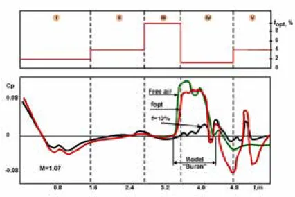
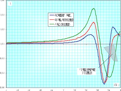
Figure 2. Optimal openness ratio distribution along the test section No 1 and pressure coefficient distribution over the wall

adaptation technology of the perforated panels of test section No 1 in the T-128 wind tunnel [2-5]

and to use it since 1986. The gist of the adaptation is following. The distributions of the flow parameters near the perforated panels (far field) were calculated for the free conditions by numerically integrating the Euler equations.

Based on the transonic area rule, the calculations were performed for the equivalent body of rotation for low incidence angles. This significantly reduced the calculation time.

During testing, pressure distributions were measured on the test section walls and were compared with computed data.

Further, the openness ratio of the panels was changed until the difference between the calculated and measured pressures reaches a minimum. Figure 2 shows the distribution of the openness ratio along the test section as well as the computed and measured pressure distributions on the walls [5]. It can be seen that the optimal distribution of the openness ratio provides an acceptable level of the pressure coefficient in the far field. The adaptation methodology at transonic flow speeds allowed one to evaluate with sufficient accuracy the maximum load acting on the attachment fitting between the Buran orbiter and the Energiya booster.

The numerical methods were also used together with the theoretical and experimental studies in the cases, when it was impossible to simulate in wind-tunnel tests all flight parameters of the Buran orbiter [6, 7]. In particular, hypersonic wind tunnels failed to simulate the air dissociation effect, which distorted the pitching moment [8].

The combination of numerical and experimental methods has provided reliable estimations of the aerodynamic characteristics at high altitudes in passing from free molecular flow to continuum as well as for heat flux with the natural laminar-turbulent transition of the boundary layer [9]. Thus, application of the numerical methods in experimental studies has allowed one to enhance the trustworthiness of the aerodynamic characteristics of the Buran orbiter for its entire flight trajectory, which was supported by a flight experiment and, as a result, ensured Buran's successful flight in the automatic mode in 1988.

The adaptation methodology was later used for testing half-models of passenger aircraft in T-128 test section No 2 [3-5].

To take into account the effect of slotted walls of test section No 3 on the airfoil profile characteristics for subsonic aircraft, a special methodology was developed [10-12] on the basis of Euler equations' potential approximation. The calculation of the turbulent boundary layer on the airfoil was based on the extension of Green's lag-entrainment method. As the boundary condition on the perforated walls, the pressure distribution measured experimentally was adopted. The computations were performed both for the free flow and in the case with perforated walls. The problem of free flow around airfoil was solved for corrected incidence angle and Mach number, so the functional representing the integral of the absolute value of the difference between computed and experimental pressure distributions over the profile surface reaches a minimum. As a result, integral corrections to the incidence angle and incoming flow Mach number were determined for free flow case with flow around airfoil being the most close to that obtainable in wind-tunnel tests.

Since 1996, to account for the effect of flow boundaries at transonic speeds, the numerical solutions of the Euler equations are being employed. The EWT (Electronic Wind Tunnel) computer code package [13-16] was developed at TsAGI. The boundary conditions at the perforated walls were presented in the form of the Darsy law (the linear relation between the normal and longitudinal components of perturbed velocity) and were determined experimentally [17, 18].

Figure 2. Optimal openness ratio distribution along the test section No 1 and pressure coefficient distribution over the wall

(3)

5^th Symposium on Integrating CFD and Experiments in Aerodynamics (Integration 2012) 3-5 October 2012

Using the EWT computer code package, the range of the fast linear method applicability [19] was determined as a function of Mach number. It turned out that for a moderate blockage of test section the linear methods can be applied up to M=0.9.

Later on, a module for numerically solving the Reynolds-averaged Navier-Stokes equations (RANS) was added to the EWT package. Presently, the code allows numerical solving stationary (RANS) and non-stationary (URANS) equations and large eddy simulation (LES). Special initial and boundary conditions are provided, such as the wind tunnel start, permeable walls (perforated and slotted), moving runway, plenum chamber, cryogenic effects, etc. As a special feature, a grid templates for different wind tunnels were created and a special block for investigated model was included. Another special block represents model support systems. An algorithm was developed for restructuring the calculation grids in accordance with variations of incidence and slip angles.

The EWT code package allows researchers to solve the three main groups of problems:

 minimization of the effect of flow boundaries (perforated walls) within the transonic speed range using the adaptive perforation technology;

 taking into account the systematic experimental errors due to flow boundary effects, support systems for complete and half-models, inherent wind-tunnel flow turbulence;

 designing the optimal contours of model support systems and panels of perforated walls to minimize flow disturbances in the test section.

Description of the EWT code computational method novel features

An in-depth description of the EWT computational method is given in [20]. The method has passed a complete evaluation and turned out to be stable in operation and providing accurate results. During the parametric computations, its algorithm was subjected to significant improvements. The flow in the wind tunnel has rather a complicated structure. It is defined by essentially viscous phenomena combined with well-developed turbulent boundary layers. Separated flow zones appear around different elements including highly deflected slats. In the case of moderate incidence angles, time-averaged approach of [20] is acceptable because the flow is stable and can be simulated numerically with the use of RANS. But there are some problems with correct prediction of drag and lift coefficients in the case of high incidence angles. Non-stationary processes connected with strong interaction between developed separation zones and non-stationary vortex sheet past the wing become essential and force to use URANS in TsAGI's computational technology [20].

Because of flow non-stationary features, one should choose explicit schemes for simulation. These schemes allow one to describe non-stationary processes with high quality. But an essential obstacle to realize such an approach is multi-scale feature of task. Characteristic times and sizes of different physical processes can differ by some orders of magnitude. Therefore, implementation of explicit schemes leads to extremely large calculation time. Contrary to that, implicit schemes are good for multi-scale problems but they show poor quality of non-stationary processes description.

A possible way to resolve this contradiction is to use zonal method. In this method, flow zones with very small scales of physical processes (mainly, inner zones of boundary layers) are calculated using an implicit scheme, while the other part of flow is calculated using explicit one. As a result, non-stationary processes in inviscid core of flow are simulated with a high quality. In the inner part of boundary layers, an implicit scheme is used and one may hope for good results, because the information has to be transmitted across the boundary layer and non- stationary processes in the inner zone of the boundary layer have mainly to be determined by the laws persistent to the inviscid core of flow. This consideration reduces scheme requirements from the viewpoint of non- stationary process description quality and permits using the implicit scheme in such concrete zones.

Let’s consider an explicit scheme of the second order in time that is used for numerically solving the Euler and Reynolds equations. In this scheme, the time step is performed using a two-step predictor-corrector procedure:

(4)

1 1/2 1/2

* 1

1 * *

1/2 1/2

( ) ( ) 0,

2 ,

( ) ( ) 0.

n n n n

i i i i

n i

n n

i i

i

n n

i i i i

n i

u u F u F u

h u u

u

u u F u F u

h



  



 

  

 



 

 

  

 



Here, i is a number of calculation cell in space. Half-integer indices correspond to sides of calculation cell, n

is time step number, hi is grid step in space (cell size), n is a time step value. The used scheme belongs to Godunov-type class. Therefore, to calculate parameters on sides of cells, a Riemann problem solution about decay of an arbitrary discontinuity is used:

1/2( ) ( 1/2)

i i

F_ u F U_ , Ui_1/2 Decay( , )u uL R .

To achieve the second approximation order in space, a linear reconstruction of space distribution of parameters over cell is used:

2ⁱ

L i

i

h u u u

x

 

     , 1 ¹ 1 2ⁱ

R i

i

h u u u

x

 



 

     .

To calculate gradients of parameters in the cells, TsAGI-developed minimal derivative principle (MUSCL) is used. Details can be found in [1].

Such explicit scheme is stable, when time step  satisfies the known Courant-Friedrichs-Levi condition:

CFL | ( ) | 1

| ( ) |

n stab i

i n i

i i

a u h

h a u

  

     ( ) dF

a u  du .

Advantages of the scheme above are clear due to physical sense and small errors. They make this scheme optimal for high-quality description of non-stationary processes. However, attempt to use this scheme for description of flow with turbulent boundary layers was unsuccessful.

Because the velocity dx ( )

dt a u is known, the information propagates per one time step as CFLihi_{, where}

CFLi i ⁿ i

a h

  is local Courant number. A standard approach for time stepping (global time stepping) is the

following. The most rigid condition for time stepping ( min min i^stab i

   ) is used for global calculations (Figure 3а). It is typical for strongly non-uniform grids that _min _max max i^stab

   i  . It means that Courant number

min min

CFLi i stab 1

i i

a h

 

   _in

most cells. Therefore, the information propagates very slowly over the computational domain and a lot of time steps are necessary to describe the characteristic interval of global flow changing. This is the well- known problem of small time steps.

On the other hand, an implicit scheme permits one to perform the calculation with arbitrarily large values of time steps and to achieve the result immeasurably Figure3. Global, local and fractional time stepping Figure 3. Global, local and fractional time stepping

(5)

faster. This factor makes implicit schemes so popular. But, as it is shown in [20], the payment for the velocity of result obtaining is loss of non-stationary process description quality. There are some methods to accelerate the calculation in the case of explicit approach to approximation of equations. When a stationary flow is calculated using time-marching method, we aren’t interested in a quality of intermediate non-stationary process description. Only its convergence to a correct stationary state is important. In this case, different methods of convergence acceleration may be used. One of them is a method of local time stepping. It is a known approach (see, for example, [21]). In this case, the calculation in each cell is performed with time step that is defined by local restrictions in this cell (Figure3a). As a result, the time step value changes from one cell to another. But when all the parameters uiⁿ^¹ are given, they are formally prescribed to the same time layer. Later on, this procedure is repeated up to the moment, when a stationary solution is achieved. In the framework of this procedure, convergence to stationary solution accelerates essentially. The flow faster adapts to the stationary boundary conditions. It is easy to understand that the number of time steps should be Omax/min times less in comparison with global stepping. If non-stationary flow is calculated and it is important to describe each moment of this flow development correctly, then neither local time stepping nor multigrid method are acceptable. In the current work, a method of fractional time stepping is proposed. The idea of fractional time stepping is that the calculation in each cell is performed with the greatest time step (i.e. with maximal possible Courant number). But the numbers of local time steps are different in different cells and they are chosen so as all the cells achieve the same layer of physical time at some moments (Figure 3b). When the same time layer is achieved, let’s name it as a completion of global time step. For example, if a local time step in the cell A is equal to max_{, in B -}_max/ 2 and in C - max/ 8, then, during one global time step, one should perform one local time step in the cell A, two local time steps in the cell B and eight local time steps in the cell C. Therefore, the global time step in each cell is divided (fragmented) into smaller local time steps so as the local time steps satisfy the local restriction on time step in the given cell. That’s why the procedure is named fractional time stepping.

It should be noted that the first description of such method is known from [22]. Let’s consider fractional time stepping organization in details. Before beginning of the calculation, the maximal possible value of time step (i^stab ) is determined in each cell of computational domain. Then, the maximal time step in the whole computational domain ( _max max i^stab

i

   ) is determined. Then, the value of local time step is determined in each cell. The time step value in the cell with the number i is taken equal to ^max

2

i l

  . The integer-valued parameter

l is chosen so as local stability condition ( 2

stab i stab

i i

    ) is satisfied in the given cell. As a result of this procedure, the whole collection of computational domain cells is divided into some subsets that will be named as levels. In all the cells of m-level, the value of local time step is equal to ^max

2

i M m

   _ _{, where}M is the number of levels. In the cells of the first level, the local time step is minimal; it is equal to i max in the cells of M- level. Let’s emphasize that, because the time step in each cell is defined by local time-dependent conditions of flow, the procedure of dividing the cells into the levels is performed before each global time step. During one global time step, 2^{M m}^ local time steps are performed in the cell of m-level. The number of local time steps is different in different cells. But towards the end of the global time step, time in all the cells increases by the same value - max. As a result, non-stationary development of flow is correct. This procedure diminishes total calculation time in rational programming (because few time steps is performed in large cells) and guaranties that the local value of stability coefficient (Cstab0.5;1) is used in each cell.

Now we dwell on practical aspects of implementation of implicit schemes. Let’s consider such scheme in the near-wall zone of boundary layers. The scheme must be “time-accurate” and approximate the space operator similar to explicit one. This can be written as

1 1 1 1

1/2 1/2

1 1 1

( ) ( )

1 ⁿ ⁱⁿ ⁱⁿ ⁿ ⁱⁿ ⁱⁿ ⁱ ⁿ ⁱ ⁿ 0

n n n n n n i

u u u u F u F u

h

 

     

   

 

  

    

   

   

  ^.

faster. This factor makes implicit schemes so popular. But, as it is shown in [20], the payment for the velocity of result obtaining is loss of non-stationary process description quality. There are some methods to accelerate the calculation in the case of explicit approach to approximation of equations. When a stationary flow is calculated using time-marching method, we aren’t interested in a quality of intermediate non-stationary process description. Only its convergence to a correct stationary state is important. In this case, different methods of convergence acceleration may be used. One of them is a method of local time stepping. It is a known approach (see, for example, [21]). In this case, the calculation in each cell is performed with time step that is defined by local restrictions in this cell (Figure3a). As a result, the time step value changes from one cell to another. But when all the parameters uiⁿ^¹ are given, they are formally prescribed to the same time layer. Later on, this procedure is repeated up to the moment, when a stationary solution is achieved. In the framework of this procedure, convergence to stationary solution accelerates essentially. The flow faster adapts to the stationary boundary conditions. It is easy to understand that the number of time steps should be Omax/min times less in comparison with global stepping. If non-stationary flow is calculated and it is important to describe each moment of this flow development correctly, then neither local time stepping nor multigrid method are acceptable. In the current work, a method of fractional time stepping is proposed. The idea of fractional time stepping is that the calculation in each cell is performed with the greatest time step (i.e. with maximal possible Courant number). But the numbers of local time steps are different in different cells and they are chosen so as all the cells achieve the same layer of physical time at some moments (Figure 3b). When the same time layer is achieved, let’s name it as a completion of global time step. For example, if a local time step in the cell A is equal to max_{, in B -}_max/ 2 and in C - max/ 8, then, during one global time step, one should perform one local time step in the cell A, two local time steps in the cell B and eight local time steps in the cell C. Therefore, the global time step in each cell is divided (fragmented) into smaller local time steps so as the local time steps satisfy the local restriction on time step in the given cell. That’s why the procedure is named fractional time stepping.

It should be noted that the first description of such method is known from [22]. Let’s consider fractional time stepping organization in details. Before beginning of the calculation, the maximal possible value of time step (i^stab ) is determined in each cell of computational domain. Then, the maximal time step in the whole computational domain ( _max max _i^stab

i

   ) is determined. Then, the value of local time step is determined in each cell. The time step value in the cell with the number i is taken equal to ^max

2

i l

  . The integer-valued parameter

l is chosen so as local stability condition ( 2

stab

stab i

i i

    ) is satisfied in the given cell. As a result of this procedure, the whole collection of computational domain cells is divided into some subsets that will be named as levels. In all the cells of m-level, the value of local time step is equal to ^max

2

i M m

   _ _{, where}M is the number of levels. In the cells of the first level, the local time step is minimal; it is equal to i max in the cells of M- level. Let’s emphasize that, because the time step in each cell is defined by local time-dependent conditions of flow, the procedure of dividing the cells into the levels is performed before each global time step. During one global time step, 2^{M m}^ local time steps are performed in the cell of m-level. The number of local time steps is different in different cells. But towards the end of the global time step, time in all the cells increases by the same value - max. As a result, non-stationary development of flow is correct. This procedure diminishes total calculation time in rational programming (because few time steps is performed in large cells) and guaranties that the local value of stability coefficient (Cstab0.5;1) is used in each cell.

Now we dwell on practical aspects of implementation of implicit schemes. Let’s consider such scheme in the near-wall zone of boundary layers. The scheme must be “time-accurate” and approximate the space operator similar to explicit one. This can be written as

1 1 1 1

1/2 1/2

1 1 1

( ) ( )

1 ⁿ ⁱⁿ ⁱⁿ ⁿ ⁱⁿ ⁱⁿ ⁱ ⁿ ⁱ ⁿ 0

n n n n n n i

u u u u F u F u

h

 

     

   

 

  

    

   

   

  ^.

(6)

In the linear case, it can be proved that proposed scheme is absolutely stable. Formally, the time step n_{may be}

arbitrarily large (CFL1). It permits one to accelerate essentially the calculation in near-wall zones.

Different approaches to solution of such non-linear equation systems are possible. For example, it’s well-known Newton’s method. The system of equations may be presented as: R u( ⁿ^¹) 0 _{, where}

1 1 1 1

1 , 2 , ...,

n n n n

u ^  u^ u ^ uN^ ^T^,RR R1, , ...,2 RN^T, where

1 1 1 1

1/2 1/2

1 1 1

( ) ( )

1 ⁿ ⁱⁿ ⁱⁿ ⁿ ⁱⁿ ⁱⁿ ⁱ ⁿ ⁱ ⁿ

i

n n n n n n i

u u u u F u F u

R h

 

     

   

 

  

    

       ^.

As result, Newton’s algorithm may be realized as following iterative procedure:

(0)

1

( ) ( 1) ( 1) ( 1)

1 ( )

,

( ) ( ),

1, ..., , .

n

k k k k

n M

u u

u u R u R u

u

k M

u u



  



 

  

  

  

  

 

 



It is easy to see that procedure needs vast resources of RAM (it is necessary to store in RAM the matrix R u



 ⁾ and it is quite time expensive (costs per iteration are very large, the matrix above is calculated at each iteration).

That’s why the dual-time stepping method is more popular in technical applications. In the case of dual approach, a fictitious non-stationary term is added to the main equation (let’s name it as pseudo one):

1 1/2 1/2

1 1 1

( ) ( )

1 ⁿ ⁱⁿ ⁿ ⁱⁿ ⁱⁿ ⁱ ⁱ 0

n n n n n n i

u u u u F u F u

u

h

 

      

  

  

    

      

     ^.

Here,  is pseudo-time. The idea of method is quite clear: the iterative solution of the pseudo system coincides with the solution of the main system in the stationary state, uuⁿ^¹. So, the solution of the main equation can be obtained as a set of the pseudo solutions stabilized at different times. One of the first realizations of the dual- time method was proposed by E. Jameson [21]. It is written as:

(0)

( 1) ( ) ( ) 1 ( ) ( )

1/2 1/2

1 ( )

,

( ) ( )

3 1 0, 1,..., ,

2 2

,

n

i i

k k k n n n k k

i i i i i i i i

n M

i i

u u

u u u u u u F u F u

k M

h

u u

  

 



 

    

     

 

 



1/2( ( )^k ) ( 1/2)

i i

F_ u F U_ , Ui_1/2Decay( , )u uL R _,

( ) ( )

2

k k

L i

i

u h

u u

x

 

     ,

( ) ( )

1

12

k k

R i

i

u h

u u

 x



 

     .

To accelerate the convergence to the stationary state, it’s possible to use a local time stepping. It’s a quite expensive procedure. The TsAGI approach uses a highly-efficient implicit scheme with a significantly simplified implicit operator. Such a hyper-fast operator is presented below:

   

















 



 





 

 

 

 











 



 







.

, ,..., 1 , ) 0 ( )

(

~

~ 2

1 2

3 ,

) ( 1

) 2 ( / ) 1 2 ( / 1

) (1/2 )

1 (1/2 2

/ ) 1

(1/2 )

1 (1/2 2

/ 1

1 )

1 ( ) ( ) 1 (

) 0 (

M i n i

k i k i

k i k i i k i k i i

n i n i n i k i k i k i

n i i

u u

M h k

u F u F

h

U U

A U

U A

u u u u

u u





(7)

It is easy to see that the proposed scheme has the first order of approximation in pseudo-time. The implicit part of space operator is obtained using linearization. Jacobeans Ai_1/2 A u u( ,iⁿ iⁿ_1) are calculated only once for each physical step. This approach results in a system of linear algebraic equations for all the cells in computational domain. This system has banded matrix (its non-zero elements are aggregated near the main diagonal of the matrix). But, in the case of a 3D problem, this “band” is a quite wide. The elements of non-zero diagonals are blocked in matrix with size 7х7. This scheme doesn’t require essential RAM, because it uses modified Gauss- Seidel method [22] with iterative architecture.

In this modified technology [20], the computational domain is subdivided into two zones. The first one is located near walls deeply inside of boundary layer. The calculations in this zone are performed using implicit scheme with dual-time stepping. The second one contains the other part of computational area. The calculations here are performed using explicit scheme with fractional time stepping. This method allows one to pose and solve non-stationary problems associated with wind-tunnel testing.

Application of the EWT program package to T-128 transonic wind-tunnel testing

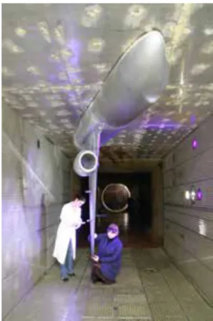
Initially, the EWT program package was adapted to the T-128 operating conditions. The application of half- models (Figure 4) in this wind tunnel allows one to reach higher Reynolds numbers (about 20⁶) corresponding to flight conditions for regional aircraft. A major methodological problem in testing half-models is the effect of the boundary layer developing on the test section wall and encountering the model's fuselage.

The influence of the boundary layer on the flow around models can be partially eliminated by employing a peniche. It is intermediate support element between the wall and the model to move it farther from the wall.

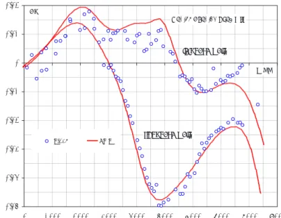
Using the EWT code package, massive computation were performed to determine the effect of the skirt-like peniche on the aerodynamic characteristics of tested half-models as well as to evaluate optimal dimensions of this support element. A numerical investigation was devoted to find out the peniche height's impact on the aerodynamic loads acting on the model. The flow past the model was computed twice. The first series was performed using different peniche heights: 17 mm, 35 mm and 70 mm. The second series was performed using the isolated model. Comparison gave estimation for the best peniche, which almost didn’t influence on the model. The boundary layer parameters were chosen so that at a certain section the computed flow velocity profile closely agreed with the experimental one (Figure 5). This section is located within the nozzle on

Figure 4. A half-model of a passenger aircraft in

T-128 test section No 2 Figure 5. Flow velocity profile in the boundary layer in the nozzle

Figure 4. A half-model of a passenger aircraft in T-128 test section No 2

Figure 5. Flow velocity profile in the boundary layer in the nozzle

(8)

the upper wall of the T-128 wind tunnel, where the velocity profile in the boundary layer was measured.

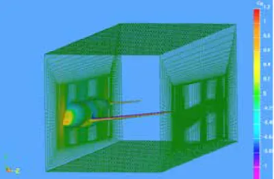
The computation grid for the half- model on the peniche of 37 mm height consisted of 411 blocks and 6.4 million nodes. The entire computational domain was divided into three parts.

The first part is the far field with a coarse computation grid. The second part is the region, where the development of the boundary layer is being modeled on the test section wall.

The third part is the surface of the semi-span model on the peniche. The greatest number of the nodes are located near the model (Figure 6).

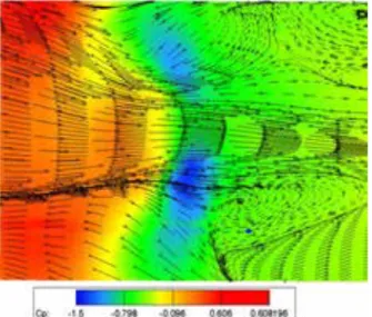
The computations were performed for M=0.78, two values of the incidence angle and two values of stagnation pressure, Pt =0.5 and 2.5 atm. Figure 7 demonstrates the computation results in terms of pressure coefficient

Figure 7. Flow about the complete model and the half-model with a peniche

distribution over the model surface and over the test section wall and streamlines on the wall without the boundary layer (the case of the complete model) and in the presence of the wall (the case of the half-model).

These computations revealed the presence of a stagnation point on the wall upstream of the fuselage and dividing streamlines outgoing from the point. Figure 8 compares the limiting streamlines on a solid wall near the model and on the peniche, which were obtained computationally and through surface oil flow visualization. The oil flow patterns confirmed the peculiarities of flow around the model fuselage revealed computationally.

Figure 8. Limiting streamlines on the solid wall near the fuselage at M=0.78 and =2.4. Computation versus visualized experiment

Figure 6. Computation grid on the model and the test section walls Figure 6. Computation grid on the model and the test section walls

Figure 8. Limiting streamlines on the solid wall near the fuselage at M=0.78 and α=2.4°. Computation versus visualized experiment

Figure 7. Flow about the complete model and the half-model with a peniche

(9)

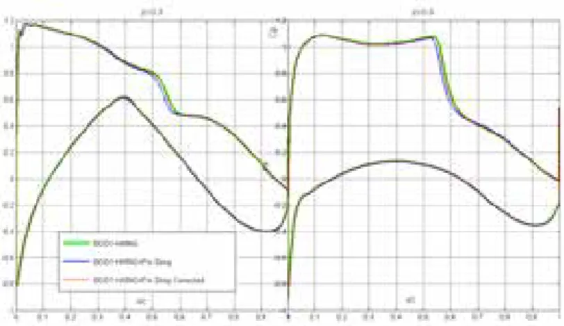
Figure 10. Comparison of pressure distributions at two wing sections for a model with and without a fin sting. Corrected pressure data are given for the model with the fin sting

Figure 9 demonstrates the effect of the peniche height on pressure coefficient in terms of the difference between the drag coefficients for the complete model and the half-model with peniche. The computational results show that the optimal height for the T-128 environment is about 35mm, which correspond to twice the boundary layer displacement thickness, 2^, on the test section wall at the location of the model.

Similar optimal height of peniche was obtained in Refs. [23, 24]. The computer analysis has allowed one not only to determine the corrections for the effect of the test section wall carrying the model and its peniche, but also to evaluate the optimal height of the peniche. To obtain the optimal

height experimentally would be extremely laboring and time consuming compared to computations.

Another important area of application of numerical methods in behalf of T-128 experiments is the studies into the effect of the model support devices and permeable flow boundaries. In wind tunnel testing, aircraft models employ support systems of different types; because of this, the test conditions differ from real flight conditions.

The support devices disturb flow near the model and distort the measurements of its aerodynamic characteristics. In addition, depending on the type of support devices, the shape of models also varies in one way or another, which is must be taken into consideration. There are two important aspects in the problem on the support devices' effect:

 Direct measurement of the influence of support devices on the tested models and correction of experiment results.

 Design of support devices' aerodynamic contours to minimize their effects on the aerodynamic characteristics of models under testing.

The T-128 wind tunnel is fitted with a set of support systems of different types including straight and fin stings.

In assessing the effect of support devices, integral corrections to incidence angle and Mach number of incoming flow must first be determined. Since the model wing is the element most sensitive to these parameters, the integral corrections are determined for

the 25% MAC. Next, numerical computations are performed for two configurations of the model: with the support system and without it. For the isolated model, the required parameters of the free-stream flow are specified, whereas for the model with the support device the incidence angle and Mach number are given with the aid of preliminary computations and corrections. The differences between the aerodynamic coefficients obtained numerically for the two configurations constitute the corrections for the effect of the support system. Pressure coefficient distributions at two wing sections are compared in Figure 10.

Fuselage+Wing+Horizontal Tail

-0.0006 -0.0004 -0.0002 0 0.0002 0.0004 0.0006 0.0008 0.001 0.0012 0.0014 0.0016

-2 -1.5 -1 -0.5 0 0.5 1 1.5 2 2.5 3



CD

M=0.78 Po=0.5 bar h=35 mm M=0.78 Po=2.5 bar h=35 mm M=0.78 Po=0.5 bar h=17 mm M=0.78 Po=2.5 bar h=17 mm M=0.78 Po=0.5 bar h=70 mm M=0.78 Po=2.5 bar h=70 mm

Figure 9. The effect of the peniche height on the drag coefficient of the fuselage-wing-horizontal tail model Figure 9. The effect of the peniche height on the drag coefficient of

the fuselage-wing-horizontal tail model

Figure 10. Comparison of pressure distributions at two wing sections for a model with and without a fin sting. Corrected

pressure data are given for the model with the fin sting

(10)

Computations are made for the model with a fin sting and without it. The data with the fin sting taken into consideration are given with corrections to incidence angle and Mach number and with no corrections. The effect of the fin sting is seen as an upstream displacement of the pressure shock. Using the obtained integral correction, it was possible to ensure the flow around the wing corresponding to the isolated model.

The numerical results furnish insights into the nature of the flow in the area of the fuselage-straight sting joint.

Figure 11 demonstrates streamlines in the internal cavity of the fuselage and the pressure distribution over the sting surface and the internal surface of the fuselage. The gas in the internal cavity is practically stagnant. It confirms the hypothesis put forward in the 1940s on the pressure constancy within the cavity. Based on this hypothesis, the correction is defined for the base drag in wind tunnel testing. In the area of the sting- fuselage joint, a complicated vortical flow is observed.

The possibility of numerically determining the corrections for the effect of support devices also allows one to use these corrections for aerodynamic design.

This problem is similar to the aerodynamic design of aircraft and their components. With this in mind, for testing the passenger aircraft configurations in the T- 128, an optimal fin sting was designed (the middle one in Figure 12). The initial version was an available Base fin sting (the lower one in Figure 12). Parametric computations were performed for different positions and configurations of the sting elements. Figure 13 shows the distribution on the fuselage side of the difference between the pressure coefficients for the configurations with and without sting. Besides, the Figure 13 also demonstrates the effect of the fin (there are data for the model with and without fin). The optimal fin sting provides the pressure distribution close to that produced by the model fin. Based on the analysis, a version was selected with the lowest effect

on the aerodynamic characteristics of the passenger aircraft model under study and meeting strength requirements.

For assessing the effect of the porous boundaries on models' characteristics in the T-128 wind tunnel, in parallel with using the linear aerodynamics methods [19], the Euler equations and Reynolds- averaged Navier-Stokes equations were numerically solved. Most often the numerical methods were used to support large-scale half-models' testing (Figure 4). Presently, a Darcy-type boundary condition is specified at the external edge of the boundary layer on the perforated walls of the test section.