Towards a tensionless string field theory for the N=(2,0) CFT in d = 6

Towards a tensionless string field theory for the N=(2,0) CFT in d = 6

Author Sudarshan Ananth, Stefano Kovacs, Yuki Sato, Hidehiko Shimada

journal or

publication title

Journal of High Energy Physics

volume 2018

number 135

year 2018‑07‑20

Publisher Springer Berlin Heidelberg Rights (C) 2018 The Author(s).

Author's flag publisher

URL http://id.nii.ac.jp/1394/00000771/

doi: info:doi/10.1007/JHEP07(2018)135

JHEP07(2018)135

Published for SISSA by Springer

Received: June 5, 2018 Accepted: July 4, 2018 Published: July 20, 2018

Towards a tensionless string field theory for the N = (2, 0) CFT in d = 6

Sudarshan Ananth,^a Stefano Kovacs,^b Yuki Sato^c,d and Hidehiko Shimada^e

aIndian Institute of Science Education and Research, Dr. Homi Bhabha road, Pune 411008, India

bDublin Institute for Advanced Studies, 10 Burlington Road, Dublin 4, Ireland

cDepartment of Physics, Nagoya University, Chikusaku, Nagoya 464-8602, Japan

dDepartment of Physics, Faculty of Science, Chulalongkorn University, Thanon Phayathai, Pathumwan, Bangkok 10330, Thailand

eMathematical and Theoretical Physics Unit, Okinawa Institute of Science and Technology, 1919-1 Tancha, Onna-son, Okinawa 904-0495 Japan

E-mail: [email protected],[email protected], [email protected],[email protected]

Abstract: We describe progress in using the field theory of tensionless strings to arrive at a Lagrangian for the six-dimensional N = (2,0) conformal theory. We construct the free part of the theory and propose an ansatz for the cubic vertex in light-cone superspace.

By requiring closure of the (2,0) supersymmetry algebra, we fix the cubic vertex up to two parameters.

Keywords: Conformal Field Theory, Field Theories in Higher Dimensions, M-Theory, String Field Theory

ArXiv ePrint: 1805.10297

JHEP07(2018)135

Contents

1 Introduction 2

2 Symmetries and notation 5

3 The free theory 6

3.1 Chiral derivatives, supersymmetry and level-matching 7

3.2 Generators 8

4 The interacting theory: overlap and insertions 10

5 Ansatz for cubic interaction terms 12

5.1 Power counting in SFT 13

5.2 Computation of commutators 15

6 Conclusions and discussion 18

A Tensors with R-symmetry and spinor indices 22

A.1 R-symmetry USp(4) 23

A.2 Light-cone little group SO(4) 23

B Superalgebra 24

C Computation of [M^−α, M^−β] 25

C.1 Superparticle case 26

C.2 Contribution involvingx⁻(σ) in [M^−α, M^−β] 27

D Overlap and insertion 29

D.1 Insertion operator 29

D.2 Some mathematical properties of the overlap and the insertions 31

E Smearing and test functionals 34

E.1 Computation of commutators with smearing 34

E.2 Test functionals 35

E.3 Sample computation using test functionals 37

E.4 [QD, P⁻] via smearing and test functionals 39

JHEP07(2018)135

1 Introduction

The possible existence of a superconformal field theory with (2,0) supersymmetry in six dimensions was first pointed out in [1]. A string theory origin for such a conformal field theory (CFT) was proposed in [2] and the theory was then identified as a candidate for the description of the low-energy dynamics of M5-branes, important but elusive degrees of freedom (DOF) in M-theory [3]. In recent years, the theory has also played a crucial role in various developments in mathematical physics, with particular attention being devoted to the classification of BPS observables and the study of their properties both in six dimensions and, upon compactification, in lower dimensions.¹

The N = (2,0) theory is also interesting from the point of view of the theory space of quantum field theory. This space is governed by the renormalisation group flow [5] in which fixed points, i.e. conformal field theories [6], are an essential feature. It is known that six dimensions is the highest dimension of spacetime that permits a theory with superconformal symmetries [1]. The very existence of a six-dimensional CFT is surprising because power-counting makes it difficult to write down interacting theories (except for a scalar φ³ coupling, which does not satisfy the requirement of positive definiteness of the energy) involving a dimensionless constant in dimensions higher than four.

Despite the importance of the N = (2,0) theory and the attention it has attracted in recent years, there is no consensus on whether it should admit a Lagrangian formulation.

Various obstructions exist to the realisation of superconformal symmetry in a conventional six-dimensional local field theory. Several Lagrangian constructions have been proposed, including the matrix model approach involving a low-energy limit [7, 8], the dimensional deconstruction approach [9], and the decompactification limit of d = 5 maximally su- persymmetric Yang-Mills theory [10, 11]. For other proposals, see [12–17] and references therein. Another interesting approach is based on the idea of the conformal bootstrap [18], which does not rely on the existence of a Lagrangian.

Although the use of the bootstrap method may render a Lagrangian description unnec- essary, having an explicit Lagrangian formulation is desirable for a better understanding of the fundamental DOF of the (2,0) theory. Such a description would also clarify the rela- tionship of the (2,0) CFT ind= 6 to lower dimensional maximally supersymmetric theories and in particular theN = 4 super Yang-Mills (SYM) theory in four dimensions. Moreover, although the (2,0) CFT is inherently non-perturbative, as implied by its M-theory origin, a Lagrangian description should make it possible to construct reliable weak-coupling approx- imation schemes valid in special sectors and/or for special observables, such as near-BPS quantities. These ideas were exploited in [19,20] in the case of the ABJM theory [21] — the maximally supersymmetric CFT in three dimensions, associated with coincident M2-branes

— which is also intrinsically strongly coupled. In [19], using the AdS/CFT correspondence, a perturbative analysis of the spectrum in a special sector of the ABJM theory was success- fully compared to the dual AdS description provided by the pp-wave matrix model [22].

In this paper we propose developing a Lagrangian for the N = (2,0) theory in six di- mensions, using String Field Theory (SFT) in light-cone gauge. The use of light-cone gauge

1A review by G. Moore including a detailed list of references can be found in ref. [4].

JHEP07(2018)135

is key to our approach since it allows us in principle to determine the interacting theory by a fairly straightforward — albeit technically involved — closure of the supersymmetry algebra [23,24].

It has been argued that the six-dimensional (2,0) theory contains tensionless string DOF. In particular, in the M-theory construction in which the (2,0) theory describes the low-energy dynamics of a collection of M5-branes, the strings arise from M2-branes stretched between M5-branes. When the M5-branes are coincident the M2-branes reduce to closed strings in the world-volume of the M5-branes. Such strings are tensionless as their tension is proportional to the (constant) M2-brane tension times the separation between the M5-branes. While of course this construction does not imply that the fundamental DOF in the effective theory describing the world-volume dynamics of coincident M5-branes should be tensionless strings, it is certainly natural to consider such a possibility.

In the case of the four-dimensionalN = 4 SYM theory, open strings ending onN coin- cident D3-branes give rise to matrix-valued point-like DOF. Similarly, when considering a stack ofN coincident M5-branes, there areN×Nconfigurations of M2-branes ending on the M5-branes, with each cylindrical M2-brane degenerating to a closed string constrained to the six-dimensional world-volume of the M5-branes. Therefore we obtain a six-dimensional matrix-valued closed string theory, that we will formulate using the language of string field theory in light-cone gauge.

The approach that we propose in this paper is to construct directly a theory of ten- sionless strings in six dimensions, using the light-cone string field theory formalism, rather than to take the tensionless limit in a theory with tension. The main reason leading us to this choice is that the zero tension limit of an ordinary tensile string theory is prob- lematic and not well understood.² This is analogous to the case of general quantum field theories, in which taking a zero mass limit often requires careful analysis. The most appro- priate procedure to study such a limit would involve computing physical observables and then taking the limit on these. However, the conventional first quantised formulation of string theory, in our present understanding, only allows one to compute S-matrix elements, whereas the good observables in a conformal field theory such as the one we are trying to construct are expected to be local correlation functions. Since local correlators in tensile string theory are not understood and, further, S-matrix elements in the tensionless limit can be singular and at least not straightforward to define, we propose to construct the (2,0) CFT directly as a tensionless string theory in six dimensions rather than trying to define it as the tensionless limit of some string theory with tension.

The fact that the tensile strings and the (2,0) CFT should have fundamentally different natural observables also supports our choice to use a second-quantised, string field theory,

2The zero tension limit of ordinary tensile string theory has been studied by many authors in connection with higher spin gauge theories. For an overview and references see [25]. The tensionless limit of bosonic covariant SFT [26] was studied in [27], where the possibility of formulating the (2,0) CFT as the zero tension limit of SFT was also mentioned. Early work on tensionless strings includes [28–39]. Some discussions on the tensionless limit can be found in [40] and references therein.

JHEP07(2018)135

formulation.³ This formalism should prove better suited to the study of the observables of a CFT. Further support for such an approach follows from the analogy with the case of point particles. The world-line (first quantised) formalism is not straightforward for the study of massless particles, which instead are simple to describe in the field theory (second quantised) language.

Our approach may be compared to the standard treatment of Yang-Mills theory. As is well known, it is easier to work with massless Yang-Mills theory directly, rather than thinking of it as a limit of a theory of massive interacting vector particles, the essential reason being the gauge symmetry of the theory in the massless case. One of course also uses the second-quantised field theory formalism, rather than a first-quantised formulation, for Yang-Mills theory.

A particular virtue of our approach regards the dimension of the coupling constant. In traditional field theory, the dimension of the coupling constant depends on the dimension of spacetime. This renders the program of writing down an interacting d= 6 Lagrangian, in particular with the correct supersymmetry, very difficult. In contrast, the physical dimensions of the coupling constant do not depend on the spacetime dimension in SFT and therefore, in principle, no obstruction arises from power counting arguments. We elaborate on this point in section 5.1.

Another promising feature in our proposal is related to dimensional reduction. The six- dimensional (2,0) theory is expected to reduce to theN = 4 SYM theory in four dimensions when compactified on a torus. The coupling constant of the reduced theory,g_{Y M}, is given by the formula _g2¹

Y M ∼ ^R_R¹₂, whereR₁ and R₂ are the two compactification radii. Although the dependence on R1, in this formula, can be easily understood in terms of a standard Kaluza-Klein reduction, the dependence onR₂is much harder to understand in the context of an ordinary local field theory. Using (tensionless) string DOF, on the other hand, means that wrapped strings play a role in the reduction, thus introducing a distinction between the two compactification radii. This may lead to a mechanism for generating the required dependence onR2 in the formula for the four-dimensional coupling constant.

The choice of light-cone gauge allows one to focus exclusively on the physical DOF and in this gauge symmetry constraints can be more directly implemented, so that one can restrict or even determine the theory purely from symmetry considerations. This idea of determining the interacting Hamiltonian by requiring the closure of the symmetry algebra has proven extremely fruitful in the past [41–44]. In particular, the entire N = 4 SYM theory — for which the light-cone superspace formulation was first obtained in [23,45] — can be derived from closure of the superconformal algebra [46]. The action describing light- cone superstring field theory in ten dimensions has also been derived to cubic order in this way in [47–50] and the full Lorentz symmetry of the theory up to cubic order was verified in [51]. We also recall that light-cone gauge bosonic string field theory was developed in [52–

58] and a detailed study of the Lorentz invariance of the theory was presented in [53,59–64].

3The distinction between the first quantised and the second quantised formulations is important at the interacting level. For the free part, the two descriptions are directly related to each other, in particular in the light-cone gauge.

JHEP07(2018)135

Our aim is to construct an interacting theory of tensionless strings having the right amount of supersymmetry and a dimensionless coupling constant (which is a necessary condition for the scale invariance of the model) in six space-time dimensions.⁴ In this paper, we present the construction of the quadratic and cubic parts of the SFT action.

We formulate an ansatz, which we justify by using (part of) the restrictions imposed by the closure of the supersymmetry algebra. The cubic vertices that we obtain still contain two arbitrary parameters. Our construction is based upon the light-cone superspace formulation of the free particle with (2,0) supersymmetry in six dimensions [65,66].

Our approach combines features of both the light-cone formulation ofN = 4 SYM and the supersymmetric closed SFT. It is similar to the former since our aim is to formulate a theory with tensionless (massless), matrix-valued DOF and sixteen supercharges, while it resembles the latter because we are trying to construct a theory of closed strings.

This paper is organised as follows. In section 2, we review the relevant symmetries of the theory and explain our notation, with further details in appendices A and B. In section3, we introduce the string field, and give the free part, i.e. the part which is quadratic in the string fields, of the symmetry charges. In section4, we explain the notation necessary for describing the cubic interaction part, and introduce the two essential ingredients, the overlap and the insertion. Section 5 presents the ansatz for the cubic vertices, and shows that the ansatz is consistent with the supersymmetry algebra. A discussion of power counting is also presented. In section 6 we conclude with a discussion. Details involved in some of the definitions and computations are deferred to several appendices.

2 Symmetries and notation

The theory we are interested in exhibits N = (2,0) super-Poincar´e symmetry and its superconformal extension. The associated R-symmetry is USp(4) [1,67,68].

We choose the metric with signature (−,+, . . . ,+) and introduce the light-cone coor- dinates

x⁺= 1

√2(x⁰+x⁵), x⁻= 1

√2(x⁰−x⁵). (2.1) We denote the four transverse directions by x^α, α = 1,2,3,4. x⁺ plays the role of time implying that −P+ = P⁻ is the light-cone Hamiltonian. As is often done, we work on a surface defined byx⁺= 0.

An SO(4) subgroup of the original SO(1,5) Lorentz symmetry, acting on the transverse directions x^α, remains manifest. We introduce capital indices, A, B, . . . = 1,2,3,4, for the R-symmetry and lower case undotted and dotted indices, a, b, . . ., ˙a,b, . . .˙ = 1,2, to represent the SO(4)=SU(2)×SU(2) spinor indices.

The generators of the super-Poincar´e algebra split into two varieties. The kinematical generators

P⁺, Q_KaA, Pα, M^αβ, M^+α, M⁺⁻, (2.2)

4We expect that, as in the case ofN = 4 SYM in four-dimensions, the classical scale invariance is not broken by quantum effects.

JHEP07(2018)135

which do not pick up corrections in the interacting theory, and the dynamical generators

P⁻, Q_DaA˙ , M^−α, (2.3)

which do. When there is a possible ambiguity, such as in the case of the supercharges, we use subscripts, K and D, to differentiate between kinematical and dynamical generators.

Dynamical generators transform fields non-linearly, while kinematical generators act lin- early on the fields. In this light-cone formalism, the super-Poincar´e algebra imposes strong constraints on the theory, including on the Hamiltonian, P⁻. These symmetry algebra constraints are what we will use to determine the interacting Hamiltonian. The entire super-Poincar´e symmetry algebra is presented in appendix B.

We will not consider the closure of the full superconformal algebra and will instead focus on just the super-Poincar´e part of the algebra. We believe that this part of the super- algebra, together with the requirement of a dimensionless coupling constant, is sufficient to determine the ansatz. It would also be interesting to examine the entire superconformal symmetry, as was done previously for N = 4 SYM [46].

3 The free theory

Our study of the free theory begins with the superfield functional

φ^I_P+[x^α(σ), θ^aA(σ)]. (3.1)

We do not write the dependence on the time coordinate x⁺ explicitly. The string field depends on the total momentumP⁺and not on the momentum densityp⁺(σ), because the choice of the light-cone gauge condition implies thatp⁺(σ) does not depend onσ [69]. The fermionic coordinatesθ^aA carry both R-symmetry and SO(4) spinor indices. As explained in the introduction, we expect to have N ×N matrix-valued string fields when we have N M5-branes. We use indices I, J, . . . to label these matrix DOF. We will later fix a Lie algebra and assume I, J, . . . to be Lie algebra indices running from 1 to the dimension of the Lie algebra. The σ coordinate takes values in an interval of length [σ]. We choose

−[σ]/2< σ <[σ]/2. (3.2)

The length [σ] is taken to be proportional to P⁺ and the coefficient of proportionality is denoted by p⁺, i.e.

P⁺

[σ] =p⁺. (3.3)

p⁺ is a conventional constant and it is a c-number (it commutes with everything). The fermionic coordinatesθ^1A andθ^2A are related by complex conjugation,

θ^aA=B^¯abB^A¯Bθ^bB, (3.4) whereB^¯abis proportional to the-tensor. For our definition of tensor structures such as the B’s associated with the light-cone little group SO(4) and the R-symmetry group USp(4), see appendixA. We will refer to θ^1A asθand θ^2Aas ¯θbelow when appropriate.

JHEP07(2018)135

3.1 Chiral derivatives, supersymmetry and level-matching

There are two different formulations of supersymmetric theories in terms of light-cone superfields. In one approach, one uses superfields which depend only on θ (or ¯θ). For N = 4 SYM in four dimensions, this approach was introduced in [23]. The formulation of spacetime supersymmetric SFT by Green, Schwarz and Brink [47–50] also belongs to this class of models. In the other approach, one uses superfields depending on both θ and ¯θ, and certain chirality constraints are imposed, as was done for N = 4 SYM in [45]. While the former choice has the advantage of being direct, in the latter, formulae for the charges and the power-counting procedure [70] are more transparent because fermionic coordinates enter in supercovariant combinations.

We adopt the latter approach. Our superfields depend on both θ and ¯θ, i.e. θ^1A and θ^2A. We impose the fundamental chirality constraint on our superfield for each value ofσ,

d1A(σ)φ= 0, (3.5)

where the chiral derivative is defined by d_aA(σ) = δ

δθ^aA(σ) + p⁺

√2θ^bB(σ)_baC_BA. (3.6) C_BA is defined in appendixA.

One can solve the constraint (3.5), φ_P⁺(x^α, θ,θ) =¯ e^√12p+

Rθ^Aθ¯Adσ

Ψ_P⁺(x^α,θ)¯ . (3.7) Here Ψ is an arbitrary superfield depending only on ¯θ, which can be identified with the superfield in an approach analogous to [23,47–50].

The superstring field is a natural extension of the superfield for a superparticle in six-dimensional spacetime constructed in [65, 66]. If one focusses on the dependence of the string field on the zero-mode part of x(σ) and θ(σ), one obtains the superfield for the superparticle (for each value of the index I). The superfield corresponds to the tensor multiplet [67] of (2,0) supersymmetry, and gives the light-cone superfield corresponding to the N = 4 SYM theory in four-dimensions [45] upon dimensional reduction. This gives additional support to our idea that the superstring field is a natural choice for the construction of the (2,0) theory.⁵ In particular, it incorporates the self-duality property of the theory, because the tensor multiplet includes a two-form gauge field with self-dual field strength. Although our formulation is based on closed string DOF, it is nevertheless non-gravitational since the tensor multiplet does not contain any field of spin 2.

We introduce the local supersymmetry generator q_aA(σ) = δ

δθ^aA(σ)− p⁺

√2θ^bB(σ)_baC_BA, (3.8)

5In the degenerate case of a single M5-brane [71], the (2,0) CFT is conventionally believed to be a free theory of fields belonging to the tensor multiplet. PuttingN= 1 in our case also leads to a free theory with very many light degrees of freedom including the tensor multiplet associated with the zero mode. There is no immediate contradiction here since, being free, these fields are completely decoupled.

JHEP07(2018)135

which satisfies the following anti-commutation relations [q_aA(σ), q_bB(σ⁰)] =−√

2p⁺_abC_ABδ(σ−σ⁰), (3.9)

[q_aA(σ), d_bB(σ⁰)] = 0, (3.10)

[daA(σ), d_bB(σ⁰)] =√

2p⁺_abCABδ(σ−σ⁰). (3.11) Here and in the rest of the paper we use square brackets to denote both commutators and anti-commutators, depending on the Grassmann parity of the operators involved. We also define

p_α(σ) =−i δ

δx^α(σ). (3.12)

A level matching condition should be imposed on the string fields, which ensures that the state be invariant under shifts of σ. The condition is related to the requirement of global existence ofx⁻,

Z ∂x⁻

∂σ dσ= 0, (3.13)

where the bosonic contribution to∂_σx⁻ is [69]

∂x⁻

∂σ = 1

p⁺p_α∂x^α

∂σ . (3.14)

When fermionic DOF are incorporated, the level matching condition becomes Z

p_α∂x^α

∂σ −i∂θ^aA

∂σ (σ) δ δθ^aA(σ)

dσ

φ= 0 (3.15)

and we have

∂x⁻

∂σ = 1 p⁺

pα

∂x^α

∂σ −i∂θ^aA

∂σ (σ) δ δθ^aA(σ)

, (3.16)

which defines x⁻(σ) up to the zero-mode part X⁻= 1

[σ]

Z

x⁻(σ)dσ . (3.17)

3.2 Generators

We are now in a position to write down the “free” part of the various generators in our algebra. To simplify our presentation, we will use the language of the first quantised theory:

we present the various charges as operators acting on the string fields. The charges in the second quantisation formulation can be written down basically by sandwiching the first quantised charge between ¯φ andφ in the usual way.

We begin by noting that the fist-quantised Hamiltonian for the tensionless string in the light-cone gauge is simply

P⁻ = Z 1

2p⁺(p^α(σ))²dσ , (3.18)

and does not contain the usual (∂σx^α)² term which is proportional to the square of the tension [69]. This formula is unchanged even if one includes fermionic DOF. Equation (3.18)

JHEP07(2018)135

shows that, while an ordinary tensile string can be understood as a collection of harmonic oscillators, a tensionless string is a collection of free particles. Each part of the string moves independently and all terms involving ∂_σ vanish, except for the important level matching conditions (3.15) and the associated formula for the x⁻ coordinate (3.16). This makes the construction of the generators (except for M^−α) quite easy; we can start from the superparticle case [65,66] and we can then simply add theσ-dependence. These properties may be considered as a direct realisation of the idea of string bits [72,73].

For the supersymmetry charges we have Q_KaA=

Z

q_aA(σ)dσ , (3.19)

QDaA˙ = Z 1

√2qbA(σ) 1

p^+bcp^α(σ)σ^αca˙dσ . (3.20) Other Poincar´e generators include

M^+α = Z

−x^α(σ)p⁺dσ=−X^αP⁺, (3.21)

M^αβ = Z

x^α(σ)p^β(σ)−x^β(σ)p^α(σ)−i

√2 8

1

p⁺σ^αβa_c^cbC^−1ABq_aA(σ)q_bB(σ)

dσ , (3.22) and

M⁺⁻=−1

2 X⁻P⁺+P⁺X⁻

− Z i

2θ^aA(σ) δ

δθ^aA(σ)dσ . (3.23) All three Lorentz generators in (3.21)–(3.23) are kinematical. The only dynamical Lorentz generator is

M^−α = Z

x⁻(σ)p^α(σ)−1

2 x^α(σ)p⁻(σ) +p⁻(σ)x^α(σ) + i

2θ^aA(σ) δ δθ^aA(σ)

p^α(σ) p⁺ +

√2 8 ip^γ(σ)

(p⁺)²qaA(σ)qbB(σ)σ^{αγ ab}C^−1AB

dσ . (3.24)

The algebra satisfied by these generators is presented in appendix B. We have explicitly verified the commutators without taking care of ordering issues in the definition of products of operators, i.e. only at the level of the Poisson brackets. Useful formulae and an outline of the computation of the commutator [M^−α, M^−β] are presented in appendixC.

The action of the charges on the superfield does not spoil the chirality constraint (3.5) because the charges are written in terms ofq’s which anti-commute with chiral derivatives, [q(σ), d(σ⁰)] = 0. For M⁺⁻ and M^−α, which contain θ and _δθ^δ explicitly, the consistency with the chirality constraint needs to be checked. Using arguments similar to those in appendix C, one can show

[M⁺⁻, d_aA(σ)] = i

2d_aA(σ)−i∂_σ(σd_aA(σ)), (3.25)

[M^−α, daA(σ)] =−i 2

p^α(σ)

p⁺ daA(σ) +i∂σ

Z σ

−[σ]/2

p^α(σ⁰) dσ⁰−P^α 2

! daA(σ)

!

, (3.26)

JHEP07(2018)135

as a consequence of the fact that d_aA transforms as a density. This yields

[M⁺⁻, d_aA(σ)]φ= 0, [M^−α, d_aA(σ)]φ= 0, (3.27) which assures the consistency of the action of the generators with the chirality constraint.

4 The interacting theory: overlap and insertions

We now wish to introduce interactions in this formalism with the focus being on cubic interactions. We label the three strings using indices r, s= 1,2,3. String 3 is chosen to be the long one with strings 1 and 2 connecting to it or string 3 splitting into 1 and 2. The range ofσ1, σ2, σ3 is denoted by [σ1],[σ2],[σ3] respectively. We require that

[σ1] + [σ2] = [σ3], (4.1)

which also follows from the fact that [σ] is proportional to the conserved momentum P⁺, so that (4.1) is equivalent to

P₁⁺+P₂⁺=P₃⁺. (4.2)

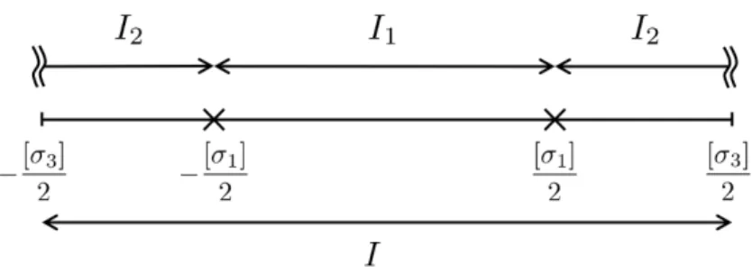
It is convenient to introduce σ which takes value in the whole interval I =I₃. The whole intervalI consists of two “intervals” I1 and I2 respectively for strings 1 and 2. We use the following scheme

I =I₃ = [−[σ₃]/2,[σ₃]/2], (4.3)

I1 = [−[σ1]/2,[σ1]/2], (4.4)

I2 = [[σ1]/2,[σ3]/2] + [−[σ3]/2,−[σ1]/2]. (4.5) Each σr takes values within [−[σr]/2,[σr]/2] for r = 1,2,3. σ and σr (r = 1,2,3) are related by

σ₃ =σ , (4.6)

σ1 =σ forσ ∈I1, (4.7)

σ2 =σ−[σ3]/2 orσ2=σ+ [σ3]/2 for σ∈I2. (4.8)

Following the work on superstring theory in the spacetime supersymmetric formal- ism [47–50], we introduce the two building blocks used to construct the cubic interactions:

the overlap and the insertions. The overlap is a delta functional connecting the third string to the first and second strings. Local insertions of operators at the interaction point are also necessary. These same ingredients (the overlap and the insertions) can be defined in the tensionless case as well.

As usual, it is easier to work with discretely labelled variables by introducing mode expansions. We introduce the Fourier components ofxr(σr) by

x_r(σ_r) =X

n

x^rne^{in[σr]2πσr}. (4.9)

JHEP07(2018)135

Figure 1. Theσ-coordinates of closed strings 1,2 and 3 are defined on intervalsI1, I2 andI=I3. The crosses indicate the interaction point.

The canonical conjugate ofxⁿ,p_n, is prn=

Z

pr(σr)e^{in[σr]2πσr}dσr (4.10) and pr0 is the total transverse momentum Pr (we omit α indices). The Fourier modes for r = 1,2 and for r = 3 respectively define two sets of basis vectors. We define a matrix A relating the basis associated with the third string to that associated with the first and second strings by

x^rn=A^rn_3mx^3m (r= 1,2). (4.11) We have

A^rn_3m = 1 [σ_r]

Z

σ∈Ir

e^{−i[σr]2πnσr}e^{+i[σ2π3]mσ3}dσ . (4.12) The overlap for the bosonic DOF is expressed as

V_B = Y

r=1,2

Y

n

δ(x^rn−A^rn_3mx^3m). (4.13) For the fermionic component, we use

V_F = Y

r=1,2

Y

a=1,2

Y

n

δ(θ^ran−A^rn_3mθ^3am). (4.14)

Our philosophy in this paper is very similar, in spirit, to that followed in [46]. In order to build a consistent interacting theory, we start with an ansatz for the dynamical supersymmetry generators. We allow the entire symmetry algebra to constrain our ansatz and finally use the fact that the Hamiltonian for the interacting theory can be written as the “square” of the dynamical supercharge.

In general, the delta function (the overlap) is not sufficient to construct the dynamical charges in light-cone gauge field theory and one has to “insert” operators such as derivatives inx and their fermionic counterparts acting on the overlap part. This is the case both for N = 4 SYM in four dimensions [23, 45] and for superstring field theory [47–50]. In string theory it is not possible to insert the operators at an arbitrary point in σ. The insertion should only act at the interaction point.

JHEP07(2018)135

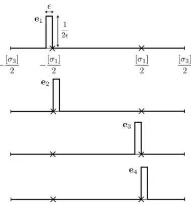
The insertion operator we choose is represented by the functions w_r(σ) (r = 1,2), which have delta function like singularities at the interaction point,

w1(σ1) =δ

σ1−[σ₁] 2

=δ

σ1+[σ₁] 2

, (4.15)

w2(σ2) =−δ

σ2−[σ2] 2

=−δ

σ2+[σ2] 2

, (4.16)

where we assume that the delta functions satisfy appropriate periodicity conditions. In the mode number representation, we have

w¹ⁿ= 1

[σ1](−1)ⁿ, (4.17)

w²ⁿ= 1

[σ2](−1)ⁿ⁺¹. (4.18)

The rationale for this choice is described in appendix D.1.

Now that we have an overlap and an insertion, we are in a position to write down an ansatz for the dynamical supersymmetry generator, describing a cubic interaction between the tensionless string fields. This is the focus of the next section.

5 Ansatz for cubic interaction terms

In general dynamical charges have an expansion, which in the case of Q_D, for instance, takes the form

Q⁽⁰⁾_D +Q⁽¹⁾_D +Q⁽²⁾_D +· · ·. (5.1) Here Q⁽⁰⁾_D is the free part, quadratic in the string fields,Q⁽¹⁾_D is the cubic interaction part, containing three string fields, and so forth. The form of the ansatz is chosen so as to satisfy the super-Poincar´e algebra (listed in appendix B) order by order in terms of the number of fields involved. The cubic part of a dynamical charge consists of two terms respectively involving φφφ and φφφ. Since one of them can be easily recovered from the other by the hermiticity conditions presented in appendixB, we will hereafter only write theφφφpart.

Our ansatz for Q⁽¹⁾_D is Q⁽¹⁾_DaA˙ =f^I_{J K}

Z φ_P+

3 I[x₃, θ₃]

×

(p_α·w)(σ^αb_a˙d_bA·w)(p⁺)^λ0(P₁⁺)^λ1(P₂⁺)^λ2(P₃⁺)^λ3δ(P₁⁺+P₂⁺−P₃⁺)V

×φ_P⁺

1

J[x1, θ1]φ_P⁺

2

K[x2, θ2]

3

Y

r=1

dP_r⁺DθrDxr. (5.2)

Here we assume thatf^IJ K are the structure constants of a Lie algebra. For the case of N M5-branes in flat spacetime, f^I_{J K} should correspond to U(N). λ0,· · · , λ3 are parameters to be determined. Below we will partially fix them by requiring invariance under rescaling

JHEP07(2018)135

of the σ coordinate and using power counting arguments. In (5.2) V =V_BV_F and pα·w=

Z

pα(σ)w(σ)dσ=pαrnw^rn, (5.3) d_bA·w=

Z

d_bA(σ)w(σ)dσ=d_bArnw^rn. (5.4) The form of the ansatz is fixed basically by requiring that it has the correct index structure.

If one exchanges r = 1 and r = 2 and the dummy indices J, K in the above formula, the result will have λ1 and λ2 exchanged. Furthermore one has a factor of −1 from each w (compare (4.15)–(4.18)) and a factor of −1 from f. This implies that we must avoid choosingλ1=λ2 to have a non-vanishing ansatz. The ansatz for P⁻⁽¹⁾ will be determined below from the supersymmetry algebra.

5.1 Power counting in SFT

We briefly discuss the power counting analysis of the cubic vertex. The first step is to notice that the appearance ofθand ¯θis accompanied by factors ofp⁺, so that the integral measure for the fermionic coordinates is dimensionless.⁶ The fermionic coordinates only contribute to the physical dimensions throughq’s andd’s and we will omit the dependence on the θ coordinates of the string field in this subsection.

The dimension of the string fields turns out to be infinite. We thus introduce a regu- larisation where we discretise the σ variables by M string bits

φ_P⁺(x^α₁,· · ·, x^α_M). (5.5) The dimension of the string field can be determined by noting that it can be considered as the wave function of the first-quantised string theory.⁷ Thus the normalisation factor

Z

|φ_P+(x^α₁,· · · , x^α_M)|²dP⁺d⁴x₁· · ·d⁴x_M, (5.6) should be dimensionless implying that the string field φhas dimension

[φ] = 1

2×(4M −1), (5.7)

which depends on the number of bits.

In the bit representation, the overlap delta functional V is V =

M1

Y

n=1

δ(x3n−x1n)

M2

Y

n⁰=1

δ x_3(M1+n⁰₎−x_2n⁰

. (5.8)

6This is because of the anti-commutation relations in superstring theory in the light-cone gauge, [θ(σ),θ(σ¯ ⁰)]∼_p¹₊δ(σ−σ⁰).

7We note that in general one can redefine the string field by multiplying it by factors of P⁺. We do not introduce such a redefinition. This choice is related to shifts of the operatorsM⁺⁻andM^−α in (3.23) and (3.24) and it is reflected in the hermitian ordering betweenX⁻andP⁺ andp⁻andx^α respectively.

JHEP07(2018)135

The schematic form (omitting factors irrelevant to the power counting) of the supercharge Q⁽¹⁾_D , after carrying out theDx1Dx2 integrals using the delta functions, is

Q⁽¹⁾_D ∼ Z ^M3

Y

n=1

d⁴x3ndP₁⁺dP₂⁺dP₃⁺φ3φ1φ2

×p·wq·wδ(P₁⁺+P₂⁺−P₃⁺) p⁺λ0

P₁⁺λ1

P₂⁺λ2

P₃⁺λ3

. (5.9)

We note that we are not introducing any dimensionful coupling constant here; this is a requirement we impose on the SFT in order to construct a scale invariant theory.

Requiring that both sides of (5.9) have dimension ¹₂, we find λ₀+λ₁+λ₂+λ₃=−3

2. (5.10)

An essential feature in the power-counting analysis of SFT presented above is that the M-dependent term in the dimension arising from the string fields

[φ₁] + [φ₂] + [φ₃] = 1

2×(4M₁−1) + 1

2×(4M₂−1) +1

2 ×(4M₃−1), (5.11) is exactly cancelled by the dimension of the measure

"_M3 Y

n=1

d⁴x_3n

#

=−4M₃, (5.12)

because of the conservation of the number of bits

M1+M2 =M3, (5.13)

for the cubic vertex.

We observe that this cancellation implies that the dimensional analysis is independent of the number of transverse directions, as can be seen from (5.11) and (5.12). This is in sharp contrast with the dimensional counting in traditional field theories. The power counting in SFT is favourable compared to that in usual QFT in this sense.

In the SFT case under consideration the free part of the action contains a term which schematically can be written as

Z

φ_P⁺(x₁, . . . , x_M)

M

X

n=1

∂

∂x^α_n 2

φ_P⁺(x₁, . . . , x_M)dP⁺d⁴x₁· · ·d⁴x_M. (5.14) Comparing this formula in the case M = M3 to the cubic vertex (5.9) we see that the terms quadratic and cubic in the fields essentially have the same structure; the difference only lies in how we group the string bits into different string fields. This is the origin of why the power counting analysis does not depend on the spacetime dimension. This in turn reflects the basic feature of string theory that locally string interaction and string propagation cannot be distinguished.

This result may have been expected as it is well known that the coupling constant in string theory is dimensionless irrespective of the spacetime dimension. The property of

JHEP07(2018)135

possessing a dimensionless coupling constant potentially makes tensionless string theory a natural framework for constructing theories with conformal symmetry.

The parameter λ₀ is fixed considering a rescaling of the σ coordinate under which [σ]

becomesα[σ]. Under this transformationp_α turns intop_α/α, i.e. it transforms as a density.

p⁺,dbA(σ), and w(σ) are also densities. Taking into account the two σ integrals involved in the definition of p·wand q·w, we see that

λ0=−2. (5.15)

Combining this with (5.10), we have

λ1+λ2+λ3 = 1

2. (5.16)

5.2 Computation of commutators

We explicitly work out the commutators to show that the ansatz is consistent with the superalgebra.

An issue in the computation is the potential singularity which can occur because of the multiplication of operators at the same point inσ-space. To perform the computations in a well defined manner we use a regularisation scheme, analogous to that introduced in [53], in which operators are smeared. For most of the commutators a computation done using smeared operators, in the limit→0 (whereis the length scale associated with smearing), produces a result which is identical to that of a formal computation without regularisation.

For the computation of the commutator [Q_D, P⁻], however, smearing makes a difference.

Also, it is necessary to evaluate the result of the computation, which includes delta func- tionals, by means of test functionals. In this section, we avoid the explicit introduction of smearing. Details regarding smearing and test functionals are discussed in appendix E.

We begin with the commutation relation,

[Q_KaA, Q_DbB˙ ] = (σ^α)_ab˙C_ABP_α. (5.17) When expanded, this implies

hQ⁽⁰⁾_K , Q⁽¹⁾_D i

= 0, (5.18)

since the kinematical generatorsQK and P have no non-linear parts.

To compute the commutator h

Q⁽⁰⁾_K , Q⁽¹⁾_D i

, we note that in general, the commutator between a symmetry generator O and the string field (at the linearised level) is given by

h

O⁽⁰⁾, φ_P⁺i

=−O ·φ_P⁺. (5.19)

Here O⁽⁰⁾ appearing on the l.h.s. denotes the linear part (quadratic in terms of the fields) of the charge in the second-quantised formulation. On the r.h.s. O· denotes how these operators act on the field (as a ket-vector) from the left in the first-quantisation formulation.

The commutator between the charges and ¯φ can be computed by taking the complex

JHEP07(2018)135

conjugate of (5.19). Apart from the case of a few exceptional operators,⁸ one can show that

hO⁽⁰⁾, φ_P⁺i

=φ_P⁺ · O , (5.20)

where ·O denotes the action of the operator from the right on the complex conjugate of the field (as a bra-vector). For instance, in the present case, we have

hQ⁽⁰⁾_KaA, φ_P⁺i

=−Q_KaA·φ_P⁺ =− Z

q_aA(σ)dσ φ_P⁺, (5.21) h

Q⁽⁰⁾_KaA, φ_P⁺i

=φ_P⁺ ·QKaA=− Z

daA(σ)dσ φ_P⁺. (5.22)

Since the operator Q⁽⁰⁾_K acts on the string fields, h

Q⁽⁰⁾_KaA, Q⁽¹⁾

DbB˙

i

=f^IJ K

Z φ_P⁺

3 I ·QKaA

(· · ·V)φ_P⁺

1

Jφ_P⁺

2

K 3

Y

r=1

dP_r⁺DθrDxr

+f^IJ K

Z φ_P⁺

3 I(· · ·V)QKaA· φ_P⁺

1

Jφ_P⁺

2

KY³

r=1

dP_r⁺DθrDxr, (5.23) where

(· · ·V) = (pα·w)(σ^αba˙dbA·w)(p⁺)^λ0(P₁⁺)^λ1(P₂⁺)^λ2(P₃⁺)^λ3δ(P₁⁺+P₂⁺−P₃⁺)V . (5.24) Using the associativity property we rewrite (5.23) as

f^I_{J K} Z

φ_P⁺

3 I Q³_KaA·(· · ·V) + (· · ·V)· Q¹_KaA+Q²_KaA φ_P⁺

1

Jφ_P⁺

2

K 3

Y

r=1

dP_r⁺Dθ_rDx_r, (5.25) whereQ^r_K withr= 1,2,3 denotes the operator Q_K acting on ther-th string field. Moving Q^1,2_K to the left of (· · ·V), (5.25) becomes

f^IJ K

Z φ_P⁺

3 I

Z

I3

qaA(σ)dσ+ Z

I1

daA(σ)dσ+ Z

I2

daA(σ)dσ

(· · ·V) φ_P⁺

1

Jφ_P⁺

2

K

×

3

Y

r=1

dP_r⁺Dθ_rDx_r. (5.26)

From this we can show Z

I3

qaA(σ)dσ+ Z

I1

daA(σ)dσ+ Z

I2

daA(σ)dσ

(· · ·V)

= X

r=1,2

Z

Ir

[d_aA(σ),(· · ·)]dσV −(· · ·) Z

I3

q_aA(σ)dσ+ Z

I1

d_aA(σ)dσ+ Z

I2

d_aA(σ)dσ

V

= 0. (5.27)

8Exceptional ones areM⁺⁻andM^−α. For these, the ordering ofθand _δθ^δ has to be worked out carefully.

JHEP07(2018)135

For the second term in the second line of (5.27), we used θ^ra(σ)−θ^3a(σ)

VF = 0,

δ

δθ^ra(σ) + δ δθ^3a(σ)

VF = 0, (5.28) whereσ ∈I_r withr= 1,2, and, for the first term,

Z

I1

w(σ)dσ+ Z

I2

w(σ)dσ= 0. (5.29)

This important property ofwis also used for the commutators [M^+α, QD] and [M^+α, P_D⁻], which can be verified using similar manipulations.

The commutator [Q_D, M^αβ] can also be verified directly. This is expected since (3.22) has the correct index structure ensuring the correct transformation ofQ⁽¹⁾_D under the SO(4) little group.

The commutation relation

Q_DaA˙ , Q_DbB˙

=√

2_a˙b˙C_ABP⁻, (5.30) yields

h

Q⁽⁰⁾_DaA˙ , Q⁽¹⁾

DbB˙

i +h

Q⁽¹⁾_DaA˙ , Q⁽⁰⁾

DbB˙

i

=√

2_a˙b˙CABP⁻⁽¹⁾. (5.31) Evaluating the l.h.s. , one obtains

P⁻⁽¹⁾ = 2√ 2 f^I_{J K}

Z φ_P⁺

3 I

(pα·w)²(p⁺)^λ0(P₁⁺)^λ1(P₂⁺)^λ2(P₃⁺)^λ3δ(P₁⁺+P₂⁺−P₃⁺)V

×φ_P⁺

1

Jφ_P⁺

2

K 3

Y

r=1

dP_r⁺DθrDxr, (5.32)

where we used

(p^α_r(σ) +p^α₃(σ))V_B= 0, (5.33) forσ ∈I_r with r= 1,2.

Commutators involvingM⁺⁻can also be verified and lead to the same condition (5.16) obtained from the power counting analysis. We note that taking the commutator of the boost generator M⁺⁻ with another operator essentially amounts to counting the number ofP⁺’s contained in the operator. One also has to take into account the “intrinsic weight”,

−¹₂, of the string field under boosts which can be read off from (3.23).

The commutator [Q_D, P⁻] = 0 requires a careful analysis using smearing and test functionals, becausep²terms inP⁻⁽⁰⁾acting on the overlap part, combined withp·winQ⁽¹⁾ may result in unwanted non-zero contributions. An outline of this calculation is presented in appendixE.4. The result justifies our choice of the insertionwexplained in appendixD.1.

The commutators involving the Lorentz generator M^−α are more subtle and we have not completed their analysis. We expect that the computation of the commutator between M^−α and P⁻ will fix the λ parameters, since the analogous parameters of the tensile superstring field theory were fixed in this way in [51].

JHEP07(2018)135

6 Conclusions and discussion

In this paper we have used light-cone string field theory to formulate an interacting theory of tensionless strings in six dimensions, with the purpose of obtaining a Lagrangian description of the (2,0) superconformal field theory. Our proposal is motivated by the M-theory picture in which the (2,0) CFT arises from the low-energy dynamics of coincident M5-branes.

In this M-theory construction, M2-branes stretched between coincident M5-branes yield degrees of freedom consisting of (matrix valued) tensionless closed strings confined to the world-volume of the M5-branes. We have argued that string field theory, in its light-cone form, is the most suitable language to study these interacting tensionless strings.

The most appealing feature of a formulation of the (2,0) CFT as a tensionless string field theory is the fact that it may allow us to avoid the obstacles, associated with power counting arguments, which impede the construction of local renormalisable interacting QFT’s in dimension larger than four. The use of stringy degrees of freedom has also interesting implications in connection with the relation between the (2,0) CFT in d = 6 and the four-dimensional N = 4 SYM theory. The latter is obtained upon dimensional reduction on a torus and we have suggested that wrapped string configurations may play a central role in the emergence of the four-dimensional Yang-Mills coupling constant.

In this paper we introduced our formalism and we presented the free part of the SFT action, together with an ansatz for the cubic interaction part. These are only the first steps towards obtaining a viable formulation of the six-dimensional (2,0) CFT. There remain multiple issues to be clarified, both of a technical nature — in the construction of the tensionless SFT — and of a more conceptual nature — in relation to its interpretation as a description of the (2,0) CFT.

In order to complete the construction of the interacting SFT to cubic order, it is important to finish the analysis of the ansatz for the M^−α Lorentz generators and their commutators with the other charges. We expect that this should allow us to completely fix our ansatz, determining the λ parameters. By a more comprehensive study of the constraints imposed by the full superconformal algebra, one can presumably deduce the full anti-symmetry and the Jacobi identity for the parameters f^I_{J K}, thus characterising them as structure constants of a Lie algebra, as was done for N = 4 SYM in [46].

Our study of the free part of the superalgebra has only been carried out at the level of the Poisson brackets, without taking care of ordering issues in the definition of operator products. It is clearly desirable to repeat these calculations at the quantum level. For this purpose it may be necessary to make a more systematic use of smearing and test functionals, following the approach discussed in appendix E.

The most important issues that remain to be addressed are, however, more conceptual and concern the interpretation of our six-dimensional tensionless SFT as describing the dynamics of the (2,0) CFT. The fundamental physical properties of a CFT formulated in this manner need to be investigated. As a theory of tensionless strings our model contains a very large number of light degrees of freedom, whose properties and behaviour need to be understood. The most crucial aspects to focus on are the identification of the correct observables in the theory and how to describe them in the SFT language. Clarifying these aspects is essential in order to understand the very nature of the resulting CFT.

JHEP07(2018)135

On general grounds, one expects the proper observables to be correlation functions of local operators organised in superconformal multiplets. Within the formulation proposed in this paper such local operators should be built from the string field. It is possible that there be a vast redundancy in our formulation, so that, in spite of the seemingly very large number of degrees of freedom contained in the string field, the set of physical observables built from them is similar to those found in more familiar conformal theories in lower dimensions. It is also possible, however, that the construction that we presented give rise to a much broader set of observables compared to more conventional CFT’s and that the system described by our tensionless string field is fundamentally different from the known examples of conformal theories.

There are several ways to gain insights into the properties of observables in the the- ory we constructed. It can be very useful to consider special sectors in which one has independent means of guessing the structure of the relevant observables. Particularly in- teresting in this respect are large R-charge states in M-theory in AdS₇ ×S⁴. According to the AdS/CFT correspondence, the (2,0) CFT has a dual description in terms of M- theory in AdS7×S⁴, which possesses a large R-charge sector analogous to that considered in [19], described by the BMN matrix model. The spectrum of the BMN matrix model includes states associated with near-BPS fluctuations of spherical membranes. Then the AdS/CFT duality implies that there exist a large R-charge sector in the six-dimensional (2,0) CFT containing operators corresponding to fluctuations of spherical membranes. Re- calling the properties of the analogous sector in the duality between type IIB string theory in AdS5 ×S⁵ and N = 4 SYM, we can speculate about the characteristics of a set of large R-charge degrees of freedom in the (2,0) CFT. In the AdS₅/CFT₄ case one consid- ers so-called BMN operators [22], which are constructed as traces of products of a large number of the matrix-valued elementary fields of the N = 4 SYM theory. The position in the sequence of fields inside such traces can be understood as being associated with the σ coordinate in the dual string. In the case of the (2,0) theory the states with large R-charge we are interested in are membrane fluctuations and thus one has two σ coordi- nates to identify in the relevant CFT operators. Since the (2,0) theory contains tensionless string degrees of freedom, it is natural to build the analog of the BMN operators as traces of products of matrix fields defined on a loop space, which is the configuration space of tensionless strings. In this way one may introduce two σ-coordinates: one associated with a given “point” in the loop space, the other labelling the order of the matrix fields in the product. Our string field precisely provides a matrix valued field on a loop space. Thus the consideration of a BMN-like sector suggests that operators written as traces of products of string fields may be a natural choice of observables in the (2,0) CFT. Although in general it is not straightforward to define a theory built on a loop space, SFT provides a rather successful example of such a theory. This is actually one of the motivations that led us to study the SFT approach proposed in this paper.

When considering the problem of identifying the observables of the (2,0) theory, it is clearly important to take into account as much as possible the constraints from sym- metry arguments and consistency requirements. The bootstrap program [18] is a way of systematically implement these constraints to obtain, in particular, bounds on the spec-