マハラザン スレンダラ

Phase Unwrapping and Directional Filtering in Magnetic Resonance Elastography of Lumbar Muscles

腰部背筋のMRエラストグラフィにおける位相アンラッピング と方向フィルタリング

2020 年 9月

東京都立大学大学院 人間健康科学研究科 博士後期課程 人間健康科学専攻 放射線科学域

マハラザン スレンダラ

別紙様式１（課程博士申請者用）

博 士 学 位 論 文

論 文 題 名

（注：学位論文題名が英語の場合は和訳をつけること。）

Phase Unwrapping and Directional Filtering in Magnetic Resonance Elastography of Lumbar

Muscles

腰部背筋の MRエラストグラフィにおける位相アンラッピングと 方向フィルタリング

（西暦） 2020 年 08 月 18 日 提出

東京都立大学大学院

人間健康科学研究科 博士後期課程 人間健康科学専攻 放射線科学域 学修番号：17997607

氏 名： マハラザン スレンダラ

（

i

注：1ページあたり1,000字程度（英語の場合300ワード程度）で、本様式1～2ページ

（A4版）程度とする。

This thesis elaborates the image processing steps (phase unwrapping and directional filtering) which are applied to the psoas major muscles in a stiffness imaging technique, known as MR elastography. Magnetic Resonance Elastography (MRE) is a dynamic MR imaging technique that can non-invasively quantify the bio-mechanical properties of soft tissues via the direct visualization and measurement of shear wave displacements, transmitted by using mechanical vibrations. MRE is an emerging and promising biomarker imaging tool for the early detection of alteration in biomechanical properties.

This thesis begins with the structure of muscles, skeletal muscle imaging and an introduction to MR elastography technique. A theoretical background regarding MR imaging and MR elastography is summarized. The fundamental concept of MRI and MRE was essential to understand the image acquisition in MRI imager and image processing steps, namely phase unwrapping and filtering, and elastogram reconstruction in MRE respectively. Phase unwrapping is an initial step for image processing in MRE. The four phase unwrapping algorithms, namely Minimum Discontinuity (MD), Laplacian-Based Estimate (LBE), Region Growing (RG) and Dilate-Erode (DE) propagate were applied to psoas major image data. MD and LBE could successfully unwrap the phase wrapped images. However, LBE yielded higher phase amplitude than MD and is recommended for phase unwrapping of psoas major MRE data. Image filtering is the second step of image processing in MRE. Image filters, namely gaussian bandpass, directional filter and combined directional-bandpass filter was applied to the phase unwrapped psoas major image data. Among all three filters applied, results showed that the directional-bandpass filter was best suited for psoas major image filtering, since it removed wave interferences, high frequency noise components and low frequency longitudinal waves and bulk motion effects. Hence, the directional-bandpass filter could potentially yield accurate elastograms, rather than using individual filter. Two wave – inversion algorithms, namely Local Frequency

Phase Unwrapping and Directional Filtering in Magnetic Resonance Elastography of Lumbar Muscles

腰部背筋のMRエラストグラフィにおける位相アンラッピングと方向フィ ルタリング

学位の種類： 博士（ 放射線 学）

東京都立大学大学院

人間健康科学研究科 博士後期課程 人間健康科学専攻 放射線科学域

学修番号：17997607

氏 名：マハラザン スレンダラ (MAHARJAN Surendra)

（指導教員名： 沼野 智一 NUMANO Tomokazu)

ii

Estimate (LFE) and Algebraic Inversion of Differential Equation (AIDE) were used for elastogram reconstruction. The stiffness value calculated by using LFE was significantly higher than the stiffness value calculated by using AIDE. Moreover, the stiffness output by using MD phase unwrapping algorithm was significantly higher than the stiffness output by using LBE phase unwrapping algorithm. However, we were unable to measure the stiffness of psoas major in vivo. So, we were unable to mention which wave – inversion and which phase unwrapping algorithm yielded accurate elasticity value of psoas major. Furthermore, a simultaneous MRE acquisition technique of psoas major (PM) and erector spinae muscle (ESM) was developed in a conventional MRI imager. Previous literature stated that the motion-encoding gradient (MEG)-like effect was in AP direction for psoas major muscle, and in this study, the MEG-like effect was resulted in RL direction for erector spinae muscle. The AP 45°

Motion-Encoding Gradient (MEG)-like effect direction at 50 Hz vibration frequency, incorporating directional filter during image processing can obtain displacement fields in both muscles, that can be used to measure stiffness of psoas major and erector spinae muscles simultaneously.

iii

Chapter 1 Introduction 1

1.1. Skeletal Muscle 2

1.2. Structure of Skeletal Muscle 3

1.3. Skeletal Muscle Imaging 5

1.4. Overview of Magnetic Resonance Elastography 6

1.5. Thesis Objectives 7

1.6. Thesis Structure 8

Chapter 2 Magnetic Resonance Imaging 10

2.1. Introduction 11

2.2. Spin, Magnetic Fields, and Relaxation 11

2.3. Image Encoding Gradients 18

2.3.1. Slice Selection Gradient 19

2.3.2. Frequency Encoding Gradient 20

2.3.3. Phase Encoding Gradient 21

2.4. K-Space and Image Formation 22

2.5. Pulse Sequence 23

2.5.1. Spin Echo (SE) Pulse Sequence 24

2.5.2. Gradient-Recalled Echo (GRE) Pulse Sequence 26 2.5.3. Echo Planar Imaging (EPI) Pulse Sequence 29

2.6. Summary 30

Chapter 3 Magnetic Resonance Elastography 31

iv

3.1. Elasticity 32

3.1.1. Stress and Strain 33

3.2. Elasticity Imaging 37

3.3. Magnetic Resonance Elastography 38

3.3.1. Types of Magnetic Resonance Elastography 40

3.3.2. Comparison of MRE with other methods 40

3.3.3. Principles of Magnetic Resonance Elastography 41

3.3.3.1. Generating Mechanical Waves 42

3.3.3.2. Imaging Wave Propagation 43

3.3.3.3. Mechanical Property Estimation 44

3.3.4. MRE Pulse Sequence 45

3.3.5. MRE Wave Imaging 46

3.3.6. Phase Unwrapping 47

3.3.7. Wave Image Filtering 48

3.3.7.1. Band-Pass Filtering 48

3.3.7.2. Directional Filtering 48

3.3.8. Shear Modulus Calculation 49

3.3.8.1. Phase Gradient 50

3.3.8.2. Local Frequency Estimation 51

3.3.8.3. Algebraic Inversion of Differential Equation 52

3.3.9. Application of MR Elastography 52

3.3.9.1. Liver 52

3.3.9.2. Brain 54

v

3.3.9.4. Skeletal Muscles 56

3.3.9.5. Cardiac 57

3.3.9.6. Other organs 58

Chapter 4 Phase Unwrapping 59

4.1. Introduction 60

4.2. Theory 62

4.2.1. Phase Unwrapping 62

4.2.1.1. Minimum Discontinuity 63

4.2.1.2. Laplacian-Based Estimate 64

4.2.1.3. Region Growing 65

4.2.1.4. Dilate-Erode Propagate 66

4.3. Materials and Methods 67

4.3.1. MRE Experiments 67

4.3.2. MRE Sequence 68

4.3.3. Image Data 70

4.3.3.1. Phantom Data 70

4.3.3.2. Psoas Major Muscle Data 70

4.3.4. Data Analysis 72

4.4. Results 73

4.4.1. Phantom Data 73

4.4.2. Psoas Major Muscle Data 74

4.5. Discussion 78

vi

4.5.1. Phantom Data 78

4.5.2. Psoas Major Muscle Data 78

4.5.3. Study Limitations 80

4.6. Conclusion 80

Chapter 5 Image Filtering 81

5.1. Introduction 82

5.2. Materials and Methods 83

5.2.1. Image Data 83

5.2.1.1. MREWave Phantom Data 83

5.2.1.2. Fruit Jelly Phantom Data 84

5.2.1.3. Psoas Major Muscle Data 86

5.2.2. MRE Experiments and MRE Pulse Sequence 86

5.2.3. Image Filters 86

5.2.3.1. Gaussian Bandpass Filter 87

5.2.3.2. Directional Filter 87

5.2.4. Data Analysis 88

5.3. Results 89

5.3.1. MREWave Phantom Data 89

5.3.2. Fruit Jelly Phantom Data 92

5.3.3. Psoas Major Muscle Data 95

5.3.3.1. Comparison of MAV for MD-unwrapped right psoas major data

100 5.3.3.2. Comparison of MAV for MD-unwrapped left psoas major

data 101

vii

data

5.3.3.4. Comparison of MAV for LBE-unwrapped left psoas major data

102 5.3.3.5. Comparison of MAV for MD-unwrapped and LBE-

unwrapped right psoas major data

102 5.3.3.6. Comparison of MAV for MD-unwrapped and LBE-

unwrapped right psoas major data 103

5.4. Discussion 103

5.4.1. MREWave Phantom Data 103

5.4.2. Fruit Jelly Phantom Data 104

5.4.3. Psoas Major Muscle Data 105

5.5. Conclusion 107

Chapter 6 Shear Modulus Calculation 108

6.1. Introduction 109

6.2. Materials and Methods 111

6.2.1. Image Data 111

6.2.2. MRE Experiments 111

6.2.3. Wave – Inversion Algorithms 111

6.2.3.1. Local Frequency Estimate 111

6.2.3.2. Algebraic Inversion of Differential Equation 112

6.2.4. Data Analysis 113

6.3. Results 114

6.3.1. MREWave Phantom Data 114

6.3.2. Fruit Jelly Phantom Data 116

viii

6.3.3. Psoas Major Muscle Data 118

6.3.3.1. Comparison of stiffness values for MD-unwrapped right

psoas major data 122

6.3.3.2. Comparison of stiffness values for MD-unwrapped left psoas major data

123 6.3.3.3. Comparison of stiffness values for LBE-unwrapped right

psoas major data

124 6.3.3.4. Comparison of stiffness values for LBE-unwrapped left psoas major data

125 6.3.3.5. Comparison of stiffness values between MD-unwrapped and

LBE-unwrapped data 126

6.4. Discussion 126

6.4.1. MREWave Phantom Data 127

6.4.2. Fruit Jelly Phantom Data 127

6.4.3. Psoas Major Muscle Data 128

6.5. Conclusion 131

Chapter 7 Simultaneous MRE acquisition of Psoas Major and Erector Spinae

133

7.1. Introduction 134

7.2. Materials and Methods 136

7.2.1. Participants 136

7.2.2. Experimental Setup 136

7.2.3. MR Elastography 137

7.2.4. Image Processing and Data Analysis 140

7.3. Results 140

7.3.1. Direction of MEG-like effect 140

ix

7.3.3. Comparison of MAV according to MEG-like effect direction 145 7.3.4. Comparison of Stiffness value according to MEG-like effect

direction 146

7.4. Discussion 149

7.4.1. Direction of MEG-like effect 149

7.4.2. Simultaneous MRE acquisition 150

7.4.3. Stiffness values, Direction of muscle fibres, and Directional Filter 152

7.4.4. Study Limitations 153

7.5. Conclusion 155

References 155

Publications 171

Conference Proceedings 172

Awards and Grants 173

Acknowledgements 174

1

Chapter 1

Introduction

2

Muscle is a soft tissue that is very much susceptible to diseases as compared to other body tissues^[1]. Early and accurate diagnosis followed by precise treatment is crucial for human life^[2]. Medical science has always been striving for identifying the most sensitive and specific diagnostic tool for various diseases, including muscle diseases^[3]. There are various imaging modalities that are currently being used in clinical practice^[4]. However, muscle imaging is still lacking as compared to other body tissues, due to poor contrast resolution^[5]. Nevertheless, with the inception of sophisticated and state-of-the-art technologies, muscle imaging has caught keen interest in recent years^[6]. Again, the cancerous and diseased muscle is relatively hard than normal muscle^[7]. Taking this into consideration, scientists are determined to distinguish cancerous and diseased muscles versus normal muscles, by using stiffness measurements^[8]. This type of imaging method dependent on biomechanical properties, such as elasticity gave birth to a new imaging technique, popularly known as elastography^[9]. Before diving into details about elastography technique, we would like to go through a conceptual understanding of muscles. Skeletal muscle is only described in the following sections because we will measure elasticity of one of the skeletal muscles.

1.1. Skeletal Muscle

Skeletal muscle, shown in Figure 1.1 is one of three types of muscles in human body, others being cardiac muscle and smooth muscle^[10]. The major functions of skeletal muscles are body movement, posture maintenance, protection and support of internal organs, regulation of sphincters and heat production^[1,10]. Elasticity is one of the characteristics of skeletal muscle^[11].

1.2. Structure of Skeletal Muscle

3

Figure 1.1 Schematic diagram of a skeletal muscle.

1.2. Structure of Skeletal Muscle

There are several levels of hierarchical structure in a skeletal muscle as shown in Figure 1.2. A whole muscle contains many fascicles^[10]. A fascicle consists of many muscle fibres, that are separated by a connective tissue. and a muscle fibre is composed of numerous muscle cells^[12–14]. Each muscle fibre is a cylindrical shaped and contains many myofibrils that consists of thick and thin cytoskeletal filaments. The thick filament consists of myosin protein, whereas the thin filament consists of actin protein. The innumerous thin filaments are connected via Z line. The area between two Z lines is known as a sarcomere.

I band is a light-appearing region that contain only thin filaments, whereas A band is a dark-appearing region that contains thick filament and overlapping thin filaments. A band contains H zone (central portion of A band) and M line (middle of H zone)^[15].During

4

muscle contraction, each sarcomere shortens as the thin filaments slide close together during muscle contraction and Z lines are pulled close together in contracted state. During relaxation, myosin head cannot contact actin molecule because the myofibrils contains regulatory proteins, namely troponin and tropomyosin, which physically covers actin.

However, when muscle fibre is excited, calcium ions (Ca²⁺) is released, that pulls the regulatory proteins aside, allowing muscle contraction^[12,13,15].

Figure 1.2 Structure of a skeletal muscle

1.3. Skeletal Muscle Imaging

5 1.3. Skeletal Muscle Imaging

The skeletal muscles imaging has not traditionally received significant attention from radiological technology. Though, the microscopic anatomy, complex physiology, and working mechanism of skeletal muscles have been well-understood for quite a long period, the difficulty in directly visualizing skeletal muscles by using conventional medical imaging technique, such as radiography might have constrained the advancement of the skeletal muscle imaging^[6]. The traditional imaging technique provided an ancillary role in diagnosis of myositis and inflammatory myopathies compared with muscle biopsy, electromyopathy (EMG), biochemical laboratory studies, and physical examination.

There are a variety of other diagnostic imaging modalities that have paved the path of muscle imaging, such as sonography and scintigraphy^[5,6]. Sonography is operator- dependent, difficulty in deep tissue structures, narrow field-of-view and limited contrast resolution, whereas scintigraphy lacks specificity^[6,16]. However, with the revolutionary improvement in digital imaging, and the establishment of cutting-edge and sophisticated cross-sectional imaging technologies, such as Computed Tomography (CT), and Magnetic Resonance Imaging (MRI), the imaging of the muscles has progressed rapidly in these few years^[17,18]. Computed Tomography (CT) imaging is limited by poor soft tissue contrast and the risk of X-ray radiation exposure^[19]. Though, CT, along with radiography, sonography, scintigraphy provides some evidences for muscle imaging, MRI is entirely sensitive for soft tissue and muscle imaging. MRI is based on the fact that the behaviour of protons placed in a strong magnetic field behave differently according to tissue composition and structure^[20]. With the recent advancement in MRI technology, functional and dynamic imaging has also become possible in clinical practice, that can be used as an alternative to invasive procedures for disease diagnosis and treatment plan.

6

Palpation has been used by clinical health professionals for centuries for the diagnosis of alteration in soft tissues^[9,21,22]. The abnormalities in soft tissues have altered tactile sensation, that can be measured by biomechanical properties, such as elasticity. Tumoral organs and fibrotic tissues, such as liver cirrhosis, brain tumours, breast cancer, prostate cancer are stiffer than normal healthy tissues^[8,23]. In clinical medical practice, doctors can easily determine the situation of the internal tissues, by applying pressure directly to the surface of the body. However, it is often impossible to palpate deep tissues and measure stiffness of the tissues by haptic sensation^[24].

Medical imaging modalities, such as radiography, CT, MRI, Ultrasound and Scintigraphy can provide the internal anatomical structure of the body. Yet, Ultrasound and MRI are currently used to compute elasticity values and are analogous to virtual palpation. This type of imaging technique is called as “Elastography”, the term coined by Ophir et al^[25]. Though, researchers are also investigating on x-ray based elastography technique, it is still under development phase^[26]. MRI technique, when synchronized with sound waves, can produce shear waves in the tissue, which can be converted into elasticity maps^[9]. This type of MRI technique is known as Magnetic Resonance Elastography (MRE) and the elasticity map, thus obtained is known as elastogram. MRE can be defined as an innovative MR imaging technique for the non-invasive quantification of bio-mechanical properties via direct visualization of shear waves propagating in soft tissues^[9,27].

1.4. Overview of Magnetic Resonance Elastography

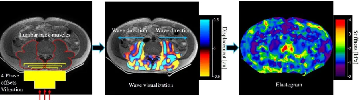
Magnetic Resonance Elastography (MRE) was invented by a group of scientists at Mayo Clinic in 1995 by Muthupillai et al^[27]. Basically, MRE involves three steps^[8,23,28]: (1) mechanical vibration of the tissue, (2) shear wave visualization and displacement

1.5. Thesis Objective

7

measurement, and (3) elastogram calculation. Figure 1.3 demonstrates the three steps required for MRE of lumbar back muscles. First of all, the muscle is vibrated by using a driver system at an apt frequency. Secondly, the motion of the tissue is visualized by using MRE pulse sequence and the displacement of the tissue can be recorded. In third step, the displacement map is converted into an elastogram by using a wave-inversion algorithm. The elastogram is the final output of MRE technique. There are various types of vibration systems, MRE pulse sequences and wave-inversion algorithms, that are presently used by various research groups. MRE technique was initially targeted to study the identification and staging of liver fibrosis^[29–32]. However, the success of MRE in liver applications has progressively led to investigation in other organs as well, such as brain^[33], breast^[34], muscles^[35], prostate^[36] and so on.

Figure 1.3 Steps required for Magnetic Resonance Elastography of lumbar back muscles.

1.5. Thesis Objectives

The primary objective of this work is to assess the different processing steps involved in MR elastography of lumbar back muscles, especially psoas major. Phase unwrapping and image filtering are applied before obtaining final elastogram by using wave – inversion algorithms. The evaluation of those processing steps and their impact on elasticity values is crucial. The most suitable phase unwrapping algorithm and image filtering are

8

determined for psoas major MR elastography. The stiffness values of psoas major and erector spinae muscle are calculated, that could be important to researchers who wish to explore further in the related field. The specific objectives of this study are given below:

1. To determine a suitable phase unwrapping method for MR elastography of psoas major muscle (Chapter 4).

2. To determine a suitable image filtering for MR elastography of psoas major muscle (Chapter 5).

3. To determine and compare the stiffness value of psoas major muscle (Chapter 6).

4. To develop simultaneous MR elastography acquisition of psoas major and erector spinae muscles (Chapter 7).

1.5. Thesis Structure

9 1.6. Thesis Structure

The introduction chapter has introduced the anatomy and physiology of muscles, importance of skeletal muscle imaging, and the fundamental concept of MR elastography.

In Chapter 2, the essential concepts and physics of Magnetic Resonance Imaging (MRI) is explained. The basic understanding of MRI is of utmost importance before diving into the notions of MR elastography (MRE). In Chapter 3, the details of elasticity, elasticity imaging, MRE, MRE pulse sequences, image processing in MRE, and application of MRE for different tissues. In Chapter 4, the phase unwrapping method and the four types of phase unwrapping algorithms, namely Minimum Discontinuity (MD), Laplacian- Based Estimate (LBE), Region Growing (RG) and Dilate-Erode (DE) Propagate, were applied to MRE image data of polyacrylamide phantom and psoas major (PM) muscle is explained. The mean amplitude value (MAV) is calculated from the phase unwrapped images for comparison. In Chapter 5, the phase unwrapped MREWave phantom, fruit jelly phantom and PM muscle images were filtered by applying bandpass filter, directional filter and combined directional-bandpass filter. The MAV was calculated for comparison. In Chapter 6, the stiffness value of MREWave phantom, fruit jelly phantom and PM muscle were computed by using two wave-inversion algorithms, namely local frequency estimate (LFE) and algebraic inversion of differential equation (AIDE). The stiffness values were compared amongst different filtered image groups and between LFE and AIDE values. In Chapter 7, the simultaneous MRE acquisition technique of PM muscle and erector spinae muscle (ESM) was developed.

10

Chapter 2

Magnetic Resonance Imaging

2.1. Introduction

11 2.1. Introduction

Magnetic Resonance Imaging (MRI) is a non-invasive method of medical imaging technique in the realm of imaging sciences^[37]. The main thrust of MRI discovery has come from the imaging of soft tissues in the human body and metabolism biomarkers.

MRI is based upon nuclear magnetic resonance (NMR) phenomenon, in which a nucleus placed in a magnetic field are perturbed by weak magnetic field and an electromagnetic signal is generated in response, with a frequency characteristic of the nucleus at the magnetic field^[37,38]. The NMR phenomenon was first discovered by Felix Bloch and Edward Purcell in 1945. In 1973, Paul Lauterbur discovered that NMR signals could be decoded into images^[39]. Again, in 1974, Peter Mansfield developed the idea of using gradients in the magnetic field for the spatial localization of NMR signal. Again, Raymond Damadian was the first to perform a full body scan of a human being in 1977 to diagnose cancer^[20].

2.2. Spin, Magnetic Fields, and Relaxation

In classical mechanics, angular momentum is the quantity of rotation of an object around an axis, which is the product of its moment of inertia and its angular velocity^[40]. There are two types of angular momenta, namely orbital angular momentum and spin angular momentum. As their names imply, each type of angular momentum corresponds to a different type of rotation: orbital angular momentum specifies orbital motion and spin angular momentum specifies spin motion^[41].

12

Figure 2.1 An atom showing electrons, revolving around a nucleus.

The results of Stern and Gerlach’s experiment in 1921^[42] resulted that both orbital motion and spin of charged particles are able to produce their own magnetic moments and can be characterized as quantum mechanical property. An atom showing electrons, revolving around a nucleus is shown in Figure 2.1. A nucleus which is electrical neutral that comprises protons and neutrons also possesses spin (𝐼 = 1/2) and possesses spin angular momentum (𝑆 = ℏ𝐼), where ℏ is Planck’s constant. However, this spin consists of a vector sum called as nuclear spin and it is also an intrinsic quantum mechanical property.

Nucleus is located at the centre of the atom; hence it has no orbital motion. For a spin rotating around an axis, magnetic moment (µ) can be related with spin angular momentum as^[43]:

µ = 𝛾𝐿 2.1

2.2. Spin, Magnetic Fields, and Relaxation

13

where γ is the gyromagnetic ratio and L is the angular momentum in the direction of magnetic moment (µ).

When the spin is placed in an external magnetic field (𝐵₀), the magnetic moment (µ) will interact with (𝐵₀), resulting in precession phenomenon against the direction of (𝐵₀) force applied with an angular velocity (𝜔₀), as shown in Figure 2.2. Precession is a change in orientation of the rotational axis of a rotating object. The angular velocity of precession (𝜔₀) can be obtained as follows^[20,44]:

𝜔₀ = 𝛾𝐵₀ 2.2

Where, 𝜔₀ is Larmor frequency, 𝛾 is gyromagnetic ratio and 𝐵₀ is magnetic field.

Furthermore, the potential energy (𝐸) is given by^[43]:

𝐸 = −µ. 𝐵₀ = −µ𝐵₀cos𝜃 2.3

14

Figure 2.2 Precession of a nuclear spin with magnetic moment (µ) about an external magnetic field B0 with an angular velocity ω0.

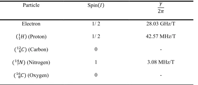
Table 2.1 shows the spin quantum number of various particles^[43]. Table 2.1 Spin quantum numbers of some common nuclei

Particle Spin(𝐼) 𝛾

2𝜋

Electron 1/ 2 28.03 GHz/T

( 𝐻₁¹ ) (Proton) 1/ 2 42.57 MHz/T

( 𝐶¹²₆ ) (Carbon) 0 -

( 𝑁¹⁴₇ ) (Nitrogen) 1 3.08 MHz/T

( 𝐶¹⁶₈ ) (Oxygen) 0 -

where, T is Tesla, SI unit of magnetic field.

The component of spin along the z-direction is as follows^[45]:

𝐿_𝑧 = h

2𝜋𝑚 2.4

Where m has 2I + 1 values, given by m = I, I – 1, I -2, …. , –I and I = ½ for a proton.

The quantized magnetic moment along the z-direction can be denoted as follows^[45]:

µ_𝑧= 𝛾 ( ℎ

2𝜋𝑚) 2.5

From equations 2.1, 2.4 and 2.5, the magnetic potential energy of the spin can be written as follows:

2.2. Spin, Magnetic Fields, and Relaxation

15

𝐸 = −µ. 𝐵₀ = −µ𝐵₀cos𝜃𝐵₀ = −𝑢_𝑧𝐵₀ = 𝛾 (hm

2𝜋) 𝐵₀ 2.6 There are two possible energy states for the magnetic moment of a proton, namely a lower and a higher energy state. To excite the spin from the lower energy state to the higher energy state, the required energy can be given as follows:

𝛥𝐸 = ℎ𝛾 ( 1

2𝜋) 𝐵₀ = ℎ𝜈_𝑅𝐹 2.7

Where, 𝜈_𝑅𝐹 is the frequency of the electromagnetic radiation. The subscript RF is radiofrequency.

𝜈_𝑅𝐹 = 𝛾 ( 1

2𝜋) 𝐵₀ 2.8

Therefore,

𝜔_𝑅𝐹 = 𝛾𝐵₀ 2.9

Where, 𝜔_𝑅𝐹 is Larmor frequency. From equation 2.2, the precession angular frequency 𝜔₀ is also equal to 𝛾𝐵₀. Hence, 𝜔_𝑅𝐹 = 𝜔₀ is the resonance condition. In 3.0 Tesla 𝐵₀ field, the Larmor frequency for the proton spin is 127.71 MHz.

16

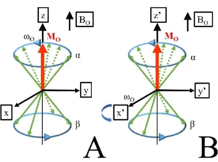
Figure 2.3 Magnetic moment, shown in a static frame of reference, A; in a dynamic frame of reference, B.

Two energy states, that is lower energy state 𝛼 and the higher energy state 𝛽 for the spins aligned along z-axis of 𝐵₀ were noted. For a small area, the spins can maintain a dynamic equilibrium along z-axis and few spins are comparatively higher in number in 𝛼 energy state than in 𝛽 energy state. The sum of the net magnetization (𝑀₀) along the direction of 𝐵₀ is as follows^[43]:

𝑀₀ = ∑ 𝑢_𝑖

𝑆

𝑖=1

2.10

Where s is the number of spins, 𝑢_𝑖 is each individual magnetic moment.

Figure 2.3A shows the static frame of reference (xyz), whereas Figure 2.3B shows the rotating frame of reference (x’y’z’) wobbling at 𝜔₀. The net magnetization 𝑀₀ is too small to be detected directly. Thus, an external magnetic field (𝐵₁) is applied

2.2. Spin, Magnetic Fields, and Relaxation

17

perpendicular to 𝐵₀, that can flip 𝑀₀ to the transverse (xy) plane, where the net magnetization can be abundantly detectable. The 𝐵₁ field is employed by using Radiofrequency (RF) pulse at Larmor frequency and 𝑀₀ can be easily detected in xy plane by placing a pair of coils in x and y axes, which can be explained by Faraday’s law of induction. The acquired MR signal is known as Free Induction Decay (FID)^[44]. The magnitude of 𝐵₁ can be expressed by an angle 𝛼⁰ and 𝑀₀ can be flipped after applying RF pulse. For 𝛼⁰ RF pulse, 𝑀₀ will flip 𝛼⁰ from longitudinal z-axis of 𝐵₀ as shown in Figure 2.4A. A 90° pulse tips 𝑀₀ down to y’ axis, with zero magnetization left in the longitudinal z-axis, as shown in Figure 2.4B. A 180° inverts down the magnetization to - z’ axis as shown in Figure 2.4C. However, the longitudinal magnetization will gradually revert to original 𝑀₀ and the transverse magnetization will decrease to zero as soon as the RF pulse is removed. The spins will retain dynamic equilibrium. This process is named as relaxation and can be divided into two independent types: spin-spin relaxation and spin-lattice relaxation.

Figure 2.4 Excitation of Net Magnetization Vector using (A) α⁰ RF pulse; (B) 90° pulse;

and (C) 180° pulse.

Spin-spin relaxation is the mechanism in which 𝑀_𝑥𝑦, the transverse magnetization decays exponentially. When the RF pulse is switched off, the local magnetic field of each spin is

18

affected by the magnetic moment from the surrounding spins. This interaction will lead to loss of phase coherence (dephasing) and a decrease in 𝑀_𝑥𝑦, which can be expressed as follows^[43]:

𝑀_{𝑡𝑟𝑟𝑜𝑡𝑎𝑡𝑖𝑛𝑔}(𝑡) = 𝑀₀sin𝛼𝑒^{−𝑡|𝑇2} 2.11

Where, 𝑀_{𝑡𝑟𝑟𝑜𝑡𝑎𝑡𝑖𝑛𝑔}(𝑡) is the transverse magnetization at time t in rotating frame of reference, 𝑀₀sin𝛼 is the transverse magnetization, and T2 decay is the time constant at which the transverse magnetization drops to 37% of its original magnitude. However, the transverse magnetization decays much faster than T2 due to additional effect of magnetic field inhomogeneities, which is known as T2* (T2 star) decay^[44].

Another relaxation type, spin-lattice relaxation recovers the longitudinal magnetization to increase from 𝑀₀cos𝛼 to 𝑀₀. This process is the result of the interaction of the spins with the lattice, that is surrounding macromolecules. The longitudinal magnetization in rotating frame of reference at time t is given as follows^[43]:

𝑀_{𝑙_𝑟𝑜𝑡𝑎𝑡𝑖𝑛𝑔}(𝑡) = 𝑀₀cos𝛼𝑒^{−𝑡/𝑇1}+ 𝑀₀(1 − 𝑒^{−𝑡/𝑇1}) 2.12 Where, 𝑀_{𝑙_𝑟𝑜𝑡𝑎𝑡𝑖𝑛𝑔}(𝑡) is the longitudinal magnetization at time t in rotating frame of reference, 𝑀₀cos𝛼 is the longitudinal magnetization, and T1 recovery is the time constant for the longitudinal magnetization to recover 63% of its initial magnetization 𝑀₀. The T1 and T2 time constants are tissue-dependent and forms the basis of image contrast.

2.3. Image Encoding Gradients

To spatially encode an image, three physical gradients are used in x, y and z directions, Gx, Gy, and Gz respectively.

2.3. Image Encoding Gradients

19

2.3.1. Slice Selection Gradient

The initial step for image encoding is slice selection, which can be performed by slice selection gradient (GSS). A magnetic field that varies linearly with slice selection plane (x, y or z) is superimposed onto the main magnetic field (𝐵₀). The Larmor frequency of the spins in a slice perpendicular to the z-axis can be written as follows^[43].

𝜔(𝑧) = 𝛾(𝐵₀+ 𝐺_𝑧𝑧) 2.13

Where, 𝜔(𝑧) is Larmor frequency at position 𝑧, 𝐺_𝑧 is the slice selection gradient along z axis.

The range of frequency within the slice can be expressed as follows^[43]:

𝛥𝜔_𝑠𝑠 = 𝛾𝐺_𝑧𝛥𝑧 2.14

Where, 𝛥𝜔_𝑠𝑠 is the frequency bandwidth of the RF pulse, and 𝛥𝑧 is the slice thickness.Thus, the thickness of the slice depends upon the bandwidth of the RF pulse and the gradient in the slice-selection gradient, as shown in Figure 2.5.

20

Figure 2.5 Slice selection gradient applied along z-axis.

2.3.2. Frequency Encoding Gradient

Frequency encoding, also known as read-out gradient (GRO) is applied perpendicular to the slice selection direction. The purpose of GRO is to make spins precess at different frequencies depending upon their position in the slice, which makes the spins spatially dependent, as shown in Figure 2.6. The magnitude of GRO depends upon Field of View (FOV) in read-out direction and Nyquist frequency. The Nyquist frequency 𝜔_𝑁𝑄 is the maximum frequency that can be sampled correctly in analog-to-digital conversion process. The read-out frequencies within a slice can be written as^[43]:

𝛥𝜔_𝑅𝑂 = 2^∗𝜔_𝑁𝑄 = 𝛾(𝐺_𝑅𝑂^∗ 𝐹𝑂𝑉_𝑅𝑂) 2.15 Where, 𝛥𝜔_𝑅𝑂 is the total range of frequencies in the image, 𝜔_𝑁𝑄 is Nyquist sampling frequency, FOVRO is the FOV along the read-out direction.

2.3. Image Encoding Gradients

21

Figure 2.6 Frequency encoding gradient applied along x-axis.

2.3.3. Phase Encoding Gradient

Phase encoding gradient (GPE) is applied perpendicular to both slice selection and frequency encoding gradients. GPE is usually applied after slice selection and before applying frequency encoding and is applied many times at different strengths in order to spatially localize the spins along the phase encoding direction. This results in different phase (𝜙) of the spins and the change in phase depends upon the magnitude and duration of GPE and the location of the spins, as shown in Figure 2.7^[41,43].

22

Figure 2.7 Phase encoding gradient applied along y-axis.

2.4. K-space and Image formation

After encoding, the image data are stored in a spatial frequency domain, known as k- space. In two-dimensional imaging, k-space is a two-dimensional grid of points, kx is related to read-out time and ky is related to amplitude of phase encoding. By using inverse Fourier transform (IFT), MR image can be obtained from k-space raw data. Each point of K-space encodes for spatial information of an entire MR image, as shown in Figure 2.8. The centre of K-space contains low spatial frequency information that contributes to the image contrast, whereas the periphery of the k-space contains high spatial frequency information that contributes to spatial resolution and image edges^[43].

2.5. Pulse Sequence

23

𝑘_𝑥 = 𝛾𝐺_𝑅0𝑡_𝑅𝑂

and,

2.16

𝑘_𝑦 = 𝛾𝐺_𝑃𝐸𝑡_𝑃𝐸 2.17

Where, 𝑡_𝑅𝑂 and 𝑡_𝑃𝐸 are the times for which the respective gradients are active.

Figure 2.8 Conventional K-space filling trajectory of signals.

2.5. Pulse Sequence

Pulse sequence is a time-line diagram of RF pulses and gradients waveforms applied during MRI signal acquisition. There are fundamental two types of pulse sequences in MRI, namely Spin Echo (SE)-based sequence and Gradient-Recalled Echo (GRE)-based

24

sequences^[43]. However, there are several other modifications of these sequences. Figure 2.9 illustrates a basic time-line diagram of a simple MRI pulse sequence.

Figure 2.9 A simple MRI pulse sequence.

2.5.1. Spin Echo (SE) Pulse Sequence

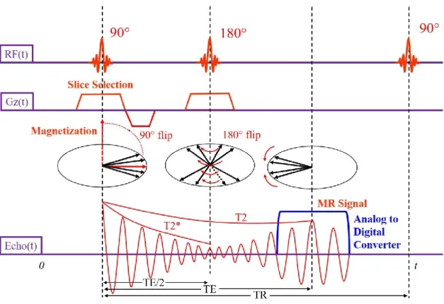
In this pulse sequence, a 90° excitation pulse flips the longitudinal magnetization into transverse plane and then a refocussing pulse of 180° will flip the transverse magnetization back into original longitudinal plane^[37]. This process will generate an echo, which is a MR signal, as shown in Figure 2.10. The time taken to generate an echo after RF excitation is called as time to echo (TE). The refocussing pulse 180° is applied exactly at half of the time taken to generate the echo after RF excitation^[37]. A reverse polarity gradient is employed in slice selection and read-out gradients to eliminate the phase dispersion caused by respective gradients^[37]. However, the reverse polarity gradient is not required in phase encoding gradient because the phase dispersion (phase shifts) are

2.5. Pulse Sequence

25

required for image encoding. A typical scan time in a two-dimensional spin echo pulse sequence can be written as^[20,43]:

𝑇_{𝑠𝑐𝑎𝑛} = 𝑇𝑅 × 𝑁_{𝑝ha𝑠𝑒}× 𝑁𝐸𝑋 2.18 Where, 𝑇_{𝑠𝑐𝑎𝑛} is the total scan time, 𝑇𝑅 is Repetition time (time period between two consecutive RF excitations), 𝑁_{𝑝ha𝑠𝑒} is the number of phase encoding steps, 𝑁𝐸𝑋 is number of excitations. A simple spin echo pulse sequence is illustrated in Figure 2.11.

Figure 2.10 Magnetization change in Spin Echo (SE) pulse sequence and generation of MR signal.

26

Figure 2.11 A simple Spin Echo (SE) pulse sequence.

T1-, T2-, and proton density (PD)-weighted images can be generated by selecting different combinations of TR and TE in SE pulse sequence, as listed in Table 2.2^[37]. Table 2.2 Image contrast according to TR and TE in SE sequence

TR Short TE Long TE

Short TR T1 weighted None

Long TR Proton density weighted T2 weighted

2.5.2. Gradient-Recalled Echo (GRE) Pulse Sequence

In this pulse sequence, a flip angle (α°) less than 90° is used and 180° refocussing pulse is not used, as shown in Figure 2.12. Hence, the scan time is reduced in GRE. Rephasing

2.5. Pulse Sequence

27

is accomplished by gradient reversal. The frequency encoding gradient is initially applied in negatively to dephase the signal, and then its polarity is reversed for rephasing, the echo thus obtained is known as gradient echo^[37,43]. The gradient waveforms do not compensate for magnetic field inhomogeneities, so the gradient echoes exhibit great deal of T2* information. A reverse polarity gradient is applied in slice selection gradient to cancel out phase dispersion^[43]. However, there is no need for reverse polarity gradient in phase encoding gradient, because the phase dispersion (phase shifts) are required for image encoding. . A typical scan time in a two-dimensional gradient recalled echo pulse sequence can be written as^[20,43]:

𝑇_{𝑠𝑐𝑎𝑛} = 𝑇𝑅 × 𝑁_{𝑝ha𝑠𝑒}× 𝑁𝐸𝑋 2.19 Where, 𝑇_{𝑠𝑐𝑎𝑛} is the total scan time, 𝑇𝑅 is Repetition time (time period between two consecutive RF excitations), 𝑁_{𝑝ha𝑠𝑒} is the number of phase encoding steps, 𝑁𝐸𝑋 is number of excitations.

28

Figure 2.12 Gradient-Recalled Echo (GRE) pulse sequence.

By manipulating flip angle (FA), TR, and TE, T1-, T2- or proton density (PD)-weighted images can be obtained, as shown in Table 2.3^[41].

Table 2.3 Image contrast according to TR and TE in GRE sequence

Flip Angle (FA) TR TE Weighting

Large FA Short TR Short TE T1

Small FA Short TR Long TE T2*

Small FA Short TR Short TE Proton density

2.5. Pulse Sequence

29

2.5.3. Echo Planar Imaging (EPI) Pulse Sequence

In this pulse sequence, a train of echoes are acquired following a single excitation within one TR cycle, as shown in Figure 2.13. EPI is the fastest pulse sequence in MRI and can be incorporated into SE or GRE pulse sequence^[41]. The phase encoding is performed by adding a constant amplitude gradient lobe or ‘blip’ after each frequency encoding gradient reversal^[37]. When the k-space is filled within one TR cycle, the acquisition is called as a Single-Shot EPI and when the k-space is filled within multiple TR cycles, the acquisition is called as a Multi-Shot EPI^[37]. EPI sequence can substantially reduce acquisition time, but image quality may be compromised^[20,37,38].

Figure 2.13 Echo Planar Imaging (EPI) pulse sequence.

30 2.6. Summary

This chapter stated the fundamental physics and basic concepts of pulse sequences accustomed to MRI. The understandings of this chapter will help readers to comprehend the principles of Magnetic Resonance Elastography (MRE), which is discussed in next chapter.

31

Chapter 3

Magnetic Resonance Elastography

32

Before we dive into details about MR elastography, it is important to understand some basic concepts regarding elasticity.

3.1. Elasticity

Elasticity is an ability of a body to resist an external force and to return to its original shape and size when that force is removed. Let’s take a simple helical spring to study its elasticity, as shown in Figure 3.1. The force required to either extend or compress the spring by some distance can be given by Hooke’s law, which states as follows^[46]:

𝐹 = −𝑘Δ𝑥 ^3.1

Where, 𝐹 is the external force, 𝛥𝑥 is the change in length along the direction of force, and 𝑘 is a real-valued number and is the elastic ability of the spring, that can be determined by the spring’s intrinsic characteristic. The negative sign indicates F as the restoring force exerted by the spring.

Figure 3.1 Hooke’ law: the force is proportional to the extension.

3.1. Elasticity

33 3.3.1. Stress and Strain

Stress is a physical quantity that expresses an internal resistance response per unit area of an object when an external force is applied to it, whereas strain is a dimensionless quantity that expresses the dimensional changes (change in shape and size) to the object. The stress (𝜎), measured in Pascal (Pa) or Newton per square meter (N/m²) can be expressed as follows^[46,47]:

𝜎 = 𝐹 𝐴

3.2

Where, F is the force applied to an area A. The strain can be written as follows:

𝜀 = 𝛥𝑙 𝑙

3.3

Where, 𝜀 is the strain, 𝑙 is the original dimension of the object and 𝛥𝑙 is the dimensional change. Again, for a linearly elastic material, for instance, the spring, Hooke’s law relates strain to stress.

𝜎 = 𝐶𝜀 ^3.4

Where, 𝐶 is a real-valued number relating strain to stress.

The 1D concept of stress can be interpreted in 3D scenario on a surface of a cube as shown in Figure 3.2.

34

Figure 3.2 A tiny cube showing stress distribution.

The internal force is indicated to x, y, and z co-ordinate axes as Fx, Fy, Fz respectively.

These internal forces produce stress at their respective planes. 𝜎_𝑖𝑗 notation is used for better understanding, where i denotes direction of normal vector for each plane and j denotes direction of vector, perpendicular to i. Therefore, there are three stresses at each plane – one parallel to the axis of stress, called as normal stress and other two perpendicular to the axis of that stress, called as shear stresses. Each internal force simultaneously produces normal and shear stresses, for example, Fz acting on plane EFGH not only produces normal stress 𝜎_𝑧𝑧, but also produces shear stresses 𝜎_𝑧𝑥 and 𝜎_𝑧𝑦 on plane CDEF and BCFG. Cauchy’s stress theorem states that we can completely

3.1. Elasticity

35

characterise stresses on each of three mutually perpendicular surfaces. These stresses form a rank two tensor, called as Cauchy stress tensor, that completely characterises the distribution of stress at a point in the material for a given stress vector t:

{ 𝑡

𝑡

𝑡

} = [

𝜎

𝜎

𝜎

𝜎

𝜎

𝜎

𝜎

𝜎

𝜎

] {

𝑛

𝑛

𝑛

}

3.5

Where, t is the stress vector and n the vector of surface unit normal, or in indicial notation:

𝑡_𝑗 = 𝜎_𝑖𝑗𝑛_𝑖 ^3.6

The stress-strain relationship is a fundamental concept in elasticity and when extended to 3D, is very complicated. According to Hooke’s law, stress 𝜎_𝑖𝑗 is related to strain 𝜀_𝑘𝑙 by a material stiffness tensor, 𝐶_{𝑖𝑗𝑘𝑙}, a four-rank tensor as:

𝜎_𝑖𝑗 = 𝐶_{𝑖𝑗𝑘𝑙}𝜀_𝑘𝑙 ^3.7

Where, 𝜎_𝑖𝑗and 𝜀_𝑘𝑙 are the second order tensor and is 𝐶_{𝑖𝑗𝑘𝑙} is the rank-4 tensor, each of the nine terms to each other for a total of 81 terms. This formula is known as Generalized Hooke’s law. Furthermore, assuming that shear stresses on the solid are equal, i.e. the cube must not be experiencing body torque, the independent stresses could be reduced to 36. The stress and strain tensors and the stiffness tensors exhibit symmetries and can be written as vectors and a matrix respectively. Using Voigt notation, the rank-4 tensor can be written into matrix as follows^[48,49]: