AN APPROACH TO SIMULATION OF PRACTICAL PROCESS
BY ANALOG COMPUTER
By
Wilson B. BENosA, Takeo FUJITA & Tadayoshi FuRuyA
(Received October 31, 1977)
SYNOPSIS
This paper presents an identification by analog computer simulation of linearized stationary model of a practical process-plastic pipe extrusion process for the control of product pipe thickness.
The mathematical model and parameters are initially constructed and estimated from the analysis of the system characteristics and process dynamics. Simulation of this model in an analog computer yields responses which satisfactorily approximate those of the actual process experi- ments,
1. INTRODUCTION
An existing plastic pipe extrusion process is taken as an example in application of identification of an actual process. Here the pipe thickness of the product pipe is desired to be controlled and kept at minimum variances under varying system disturbances.
A mathematical model is defined by a set of equations which is constructed from the analysis of system characteristics and material and energy balances, This model is then simulated in an analog computer. Separate field experiments were conducted whose data and corresponding response curves are used as basis for comparison of the simulated results. The parameters and mathematical model are adjusted to obtain as close a fitting of the response curves of the simulation results and field experiment as possible
2. PROCESS DESCRIPTION
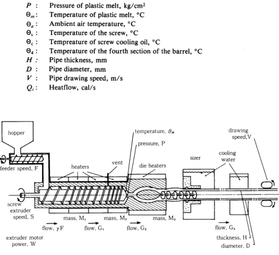
Referring to the schematic diagram of the process in Fig. 1, the following is a brief description of the extrusion process :
Plastic in powder form is loaded into a hopper and fed to the screw extruder via a screw feeder for a regulated feed rate. In the extruder, the resin is transported, compressed and heated along the barrel length. The melted resin is then extruded through a die then to a sizer where the pipe diameter is determined. The pipe is cooled then passed through a thickness measuring device.
Drawing rollers provide the transport of the pipe down to the pipe length cutter.
The following are the notations used in this paper for the different process variables :
F : Feeder Speed, rev/min S : Screw extruder speed, rev/min W : Screw extruder motor power, kW
Mi, M2, M3 : Mass at different extruder sections, kg
Gi, G2, G3 : Flow rate corresponding to Mi, M2, M3 : kg/min
-7-
P : Pressure of plastic melt, kg/cm2 e. : Temperature of plastic melt, OC
e.: Ambientairtemperature,OC es : Temperature of the screw, OC ec : Tempreature of screw cooling oil, eC
e4: Temperature of the fourth section of the barrel, OC H : Pipe thickness, mm
D : Pipe diameter, mm V : Pipe drawing speed, m/s ei: Heatflow,cal/s
hopper temperature, em drawing
speed,V
heaters Vent die heaters
-SF- . - - -
speed,S mass, Mi mass, M2 mass, M3
cooling
sizer water
"-CS2
- -- - .e-
flow, 7F fiow, Gi flow, G2 flow, G3
extruder motor thickness,H
Fig. 1: Schematic Diagram-Pipe Extrusion Process
2. 1 FIELD EXPERIMENT
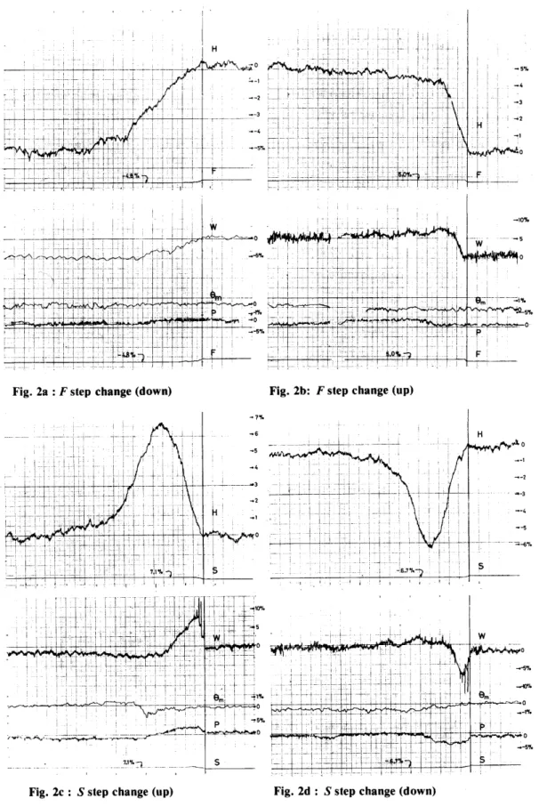
Sets of field experiments were conducted to observe the responses of some measurable process variables to step changes in Feeder Speed, F, and Screw Extruder Speed, S, and the resulting data are shown in Fig. 2. The experimental conditions are:
Fig. 2a : F step change(-4.8oro) ; S=constant Fig. 2b: F step change(+5.0cyo) ; S=constant Fig. 2c : S step change(+7.1cyo) ; F=constant Fig. 2d: S step change(---6.7oro) ; F=constant
3. SYSTEM MATHEMATICAL MODEL
3.1 PROCESS DYNAMICS
The mathematical equations that follow are derived from the process dynamics of the system which is based primarily on the kinematics of flow and storage of material and energy(i),(2)
ft M,( t)= 7f F( t)-G,( t) (1)
-StiT M2( t)= G,( t)- G,( t) (2) .
l
Fl
LP11ElFl Hx-
'
]dicV liFi-til,liitiDÅ}-i-nlibiliIlir
iFrf
--+-r
lt
K."L-
"-.-
rr -ralr[ gjl lu Iiii:IitIIl -II:Ii[i, l[ tr
tll-r1l
11.-4 a 1 T tL
- lrli]-+ L J
'I?
rL=
- Ll-
+ m
1:] i1,'rp-- 4
xit F
ei l-1ltn ,1-t I/
-r 1
i
L:
l 1" ,l --1 iv iI -" .. '"'K.",,-,•,o ,, t'i-II-l.:' i/ l' i l- li li li I
ll-.-i F tlriiTi
-.-•2 t-" I IL - i - L
,li ii :L t'Li+ #Pl` r IJ-ii . i l tr--- "J-3 r-i - l , l-, Lt-•-l --l--l -i I i
---4 1111 T-t th
rT - NF rm lrtI i-' --- -t Ul ivaii
FLI -
'i "-5't. t' f i+r uF - - L-t
Fr ---.mm"7 /L.-. i -1- luLl--
i-
J l
I/ L-LJ -I-rm um -, E
l
JV
-:i
el
L
1ii1l.i-Ii,llli[i1
- -tsvA-tO
till,ii--1ll t I`lirl
-ll:l
WM4il-.-Y.
11i[
1l 1]1
-- - l 1 ii..
I "
IT - al 1+ "
t-l Lll H' Til l It sui
- 1 14
il d
ii
t 1- T -
-"
t lL l
Ft
eu1
il1-+ilg1lt11 1i"-ii-11
11 - 1
-
t-
I" t'
rr,l.paT pu ia i g
-
t
M,-w-o pm l a l-g.- [1 , i-L -i
1 i /F
W ili ll i, 1i[ i
,L ii- -tfi--•
ii ywwi IL4
11 iilll
lt 1 i- --
l -i j ln E--tr -F-
evet :llVo 1-F t 1 H
[-".-sth iL,
1
,-L L1 -. I i i iri I i
LI
ii
-A T{ -i-1--4 i-i i I l
rll li "[lEl[
1 i -I I"F-4- tr- - F-
L L---" L, ' Lr i Å}- trr='t -, 'O Mt ,I
Fig. 2a:Fstep change (down) Fig. 2b: Fstep change (up)
-. 7V.
r"t4 I -i l . [,
t l -ln UI
' i --rl Ti- -
t
-, 5.A 1L
1.4ii[
g1 [ -3 11ik ., r[ .,
II:
o il t
l r-
il[11 IL
E
+Ai 1 sny l1 '
ill
, L
r
-.10%
- -.5
W
o [, li
-lr. Lm-m"
emi -.l y.
1 5Vo
r --ktteew-o
11
IIF
Tr-
1
F1]1l-1-•Hii
-11111lt1it-b[[li]
Iiii
1, .-J4Å}Jr'-r1]t,liF
1111[tiE,J
1 I.
--
-.-.+n
-
-.-l--m
tJi- -L
r+
1--
g.1,rrA 1l1"
ril1-i
Ilri
t-]1- l l
t
1 M--1,
gLI- ir
.Lll LtlF
-ttS
1 , 1-HFi17,IX 1tr
Lis
1.Lil ll
G 1
--1,i,1, 1itb[ iI lil tl
L
1..J7.---tr-4-
H
,-S4,
F 1
iiil1.,l
-,l.pu ,11[F11p
IIFI
ll
:lm--L-.J-
--
--
ili7iiL[i,Ll1Ll
l[+It-
ilt-,FllIi[41aiLlli!m14-
.--
11 11
ili 4II-6.7.t.
ei-L
5
--;
L4L l] 1ll L
-.-2
--,-4
--5
1rTl1 Hi[il Trl[-11 j
iV:I i-,-fr- li
IILil
l-4-
u---lt ]l r4
-r1- Fm
J-4+ii
lW,
-1ov.
.i] l '1.uI Ti[ll1 " . W
-- t T t
'LI[
1
l [liYU-1iTl
-1-it-lyT'1"t1
Lt'T
1-I--Ild1
7it-1ibm
il- ilr-1
"1
miOii}piiivFijoptl,-1li
1liv.iilli-liMt
l
--]ii rm
+-1-•-[r
1[ 1[iF-1 i'-R/eln i-11"-qi'
",lll
Wv"givo
Lfiv.
1-..lcrk
e.itz-'-.OI.-IV.
wviF-+---
o tr
-pm11:IiLil-:i--..!.tffrt:r/trrrr.--"--- p[-'5YeiH-i,t++1li "-, --t 7{r 1 -I[i- t 1
L
tF
1 rv-gp-i.o
`."stw'"y-vpt4-" "vHha-r -
tV",s--L-""J nybdwO
s
ltT+L-IF --;- '1-ILIIIil -' "+
L"rt
}rr'""--'--L
li
11-
lv1iTr-'I-1
Ig 1 i
-iLlt L 11
Fig. 2c:Sstep change (up) Fig. 2d:Sstep change (down)
Fig. 2 : Experimental Step Response-Ravv Data
-9-
ft M,( t)= G,( t)- G,( t) (3)
G,(t)=f,(S(t),M,(t)] (4)
G,( t)=f,(P( t), e.( t)) . (5) G3( t)=f3( ea(t), M3( t)] (6)
G4( t)= rp zD( t), H( t), V( t) (7)
P( t)=fp (S( t), M,( t)] (8)
VIZ(t) = f.(M,( t), M,( t), S( t)] (9) Q.( t) = (?,( t)+ (?,( t)+ (?.( t)- (?, (1 0)
(?, == o,( e, - e. )
G,
Qi = ci Gi Oi Qm =ft(c2 M2 e.)
Mi+1 Gi.1
Q. = f( M,,S)
M2 section of the extruder
Q2 = cmG2e.
Fig.3: Mass Balance Fig.4: Energy Batance
3.2 ASSUMPTIONS AND APPROXIMATIONS
At this point, the following assumptions and approximations are introduced in order to simplify the mathematical treatment :
1) that the ambient air tgmperature, e., remains constant ;
2) that the pipe diameter, D, and the pipe drawing speed, V, remain independent from the rest of the process variables since these are preset to desired values by independent devices;
3) that the powder temperature, ei, is neither a function of the feeder speed, F, nor of the screw extruder speed, S, and therefore 6ei = O;
4) that the barrel temperature at the M2 section of the extruder, e4, and the plastic melt temperature at the same extruder section, e., are approximately equal, hence, the heat flow e4 is considered nil.
At some initial equilibrium state (at t=O, designated by subscript O) when iiflM, (t) =O
Fo = Gio = G2o = G3o : 7nDoHo Vo
Taking small increments of these variables as percentages of the initial values, denote the following non-dimensional expressions
6G,
6M, =gi( t) (i= 1, 2, 3)
= mi( t)
GtoMio 6S
6H6F
Fo =f(t) so =S(t) H, =h(t)
6vaVV,=w(t) {llÅqtiLp(t) 6e.0,m=em(t)
Now simplifying Equations (1) to (10) according to the above assumptions, then expressing them in non-dimensional form, approximating in linear expression and finally taking the Laplace Transforms
Ti sMi( s)=F( s)-Gi(s) (ln) T2 sM2( s)=Gi( s)-G2( s) (2n) T3 sM3( s)=G2( s)-G3( s) (3n)
Gi( s) = KisS( s)+Ki mMi( s) e"LS (4n) G2( s) = K2pP( s)+K2 e'em( s) (5n)
G3( s) =K3 mM3( s) (6n)
G3( s) =H( s) (7n)
P(s) =- KpsS(s)+KpmM2(s) (8n)
W( s) = Ki Mi( s)+K2 M2( s)+KsS( s) (9n)
'T4 s(em( s) + M2( s)) = Ke i Gi( s) ` e.( s)
+KemM2(s)+KesS(s)"G2(s) (10n)
Note that a lag element is introduced in Egn. (4n). This is to simulate the transport lag occuring in the extruder.
3.3 PARAMETER ESTIMATION
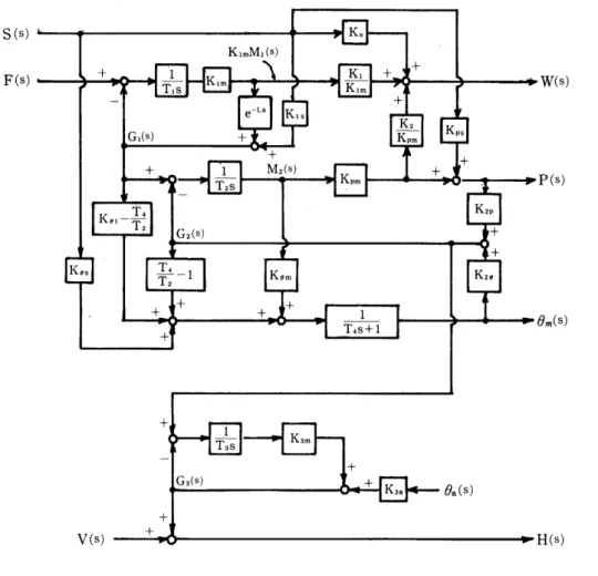
Fig. 5 is the block diagram for the simplified mathematical model described by Equations
(1 n) to (1On).
The final state conditions of the system are evaluated after step perturbations in feeder speed, F, and screw extruder speed, S, are introduced. First, consider a step change in feeder speed while the screw extruder speed is kept unchanged, then
s=o
and from Eqn. (ln) to (10n), the following steady state relations are obtained :
(F)fs = [Gi)fs =(G2]fs =(G3]fs = [H]fs (lf)
Klim= (`lk' )fs=[411L' ]fs (2f) 1=K2p(i:}]f,+K2e( iliM )f. (3f)
Kl,.= (i\-' ]f. (4f)
(i;]..= Kpm(4t' ].. (6f)
(Ill)fs = Ki (41'-]fs+ K2(4-' ]fs (7f) 1= K,, -( eFm ]f.+ K,.(\-' ]f, (sf)
-11-
S (s)
F(s)
Ks KimMi(s)
+ 1 K, + +
T,s Kim Kim
- e-Ls Kis +
G,(s)+ K,Kpm Kps
W(s
+ 1 P(s)
+M,(s)
T,s Kpm
Kei-
{l;t
-G,(s)
K2p
++
Kes T,
--T, 1 Kem K2e
- + + 1
+ T,s+1
1
em(s
H(s)
T,s K3m
+G,(s)+
K3a 0a(s)
V(s)
Fig. 5 : Simplified Block Diagram
Next, consider a step change in screw extruder speed while the feeder speed is kept unchanged, then
F=O
and again from Engs. (ln) to (10n), the following final state equations are obtained :
{l7)fs == (Gi)fs =(G2]fs =(G3]fs ==O (S)
Kis ='Kim[41/L]f, (2s)
K,p(g]f, =-K,,[ esm ]f, (3s)
K3m(ZIg't]., ..o (4s)
({}]f,=Kps+ Kpm(Ms2 ]f, (6s)
(Il;]., = Ki ('lllL' ]..+ K2 (Z!{S' ].,+ Ks (7s)
Kes =(esM]f,-Ke.(l!{i'-]f, (8s)
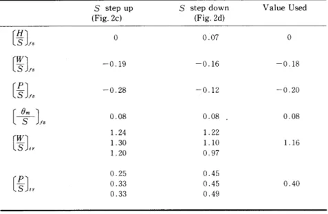
Table 1 : Transient and Final State Data (source : Fig. 2-Experiment Step Response)
F step change :
F step down F step up Value Used (Fig. 2a) (Fig. 2b)
(tll]., i.o7 i.o4 i.oo (Ill],, 1'12 1'12 1'12 (f}]f, O-41 O.39 o.4o [0I7M ]f, O.07 O.07 O
S step change :
S step up S step down Value Used (Fig. 2c) (Fig. 2d)
(ll;]., -O.19 -O.16 -o.ls
(g].. -o.2s -o.12 -o.2o (esM ).. o.os o.os. o.os
1.24 1.22
[ll;],. i.3o i.io i.i6
1.20 O.97 O.25 O.45
(g],, O•33 o.4s o.4o
O.33 O,49
From the data of the experimental results on Fig. 2, the final state and transient values of the' process variables with respect to step changes in F and S are evaluated and shown on Table 1.
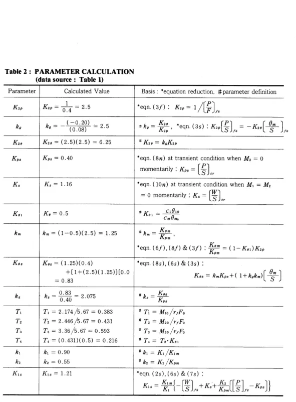
The above sets bf final state equations (Eqns. (lf) to (8f) and Eqns. (ls) to (8s) ) and the data on Table 1 form the basis for the calculations of parameters as shown on Table 2.
-13-
Table 2 : PARAMETER CALCULATION (data source: Table 1)
Parameter CalculatedValue Basis:"equationreduction,#parameterdefinition
K2p K2p=-611.ii'4=2•5 'eqn.(3f):K2p=1/(i;]f,
kg kg--( i,96g?)==2•s
#leg= ffi;,"eqn(3s):K2p(g]f,=-K2e(-(lf'L]f
K2e K2e:(2•5)(2.5)=6.25 #K2e=legK2p
Kps Kps=O.40 "eqn.(8n)attransientconditionwhenM2=O momentarily:Kps= [g],.
Ks Ks=1-16 'eqn.(10n)attransientconditionwhenMi:M2
=omomentariiy:Ks= (ll;],.
Kei Ke=O.5 #Kei=Cieiocmemo
lem km=(1'O.5)(2.5)=1.25 #k.= ffS:''eqn.(6f),(8f)&(3f):fft':l.M=(1-Kei)K2p
Kes Kes=(1•25)(O.4)
+[1+(2.5)(1.25)][O.O
==O.83
'eqn.(8s),(6s)&(3s):
Kes=kmKps+(1+kgkm)('Z;'L)
ks
O.83Nks===2.075O.40
"ks= iE':Li
ii T,=2.174/5.67=O.383 T,=2.446/5.67=O.431 T,=3.36/5.67=O.593 T,=(O.431)(O.5)=O.216
#Ti=Mio/rfFo#T2=M2o/rfFo#T3=M3o/rfFo#T4=T2'Kei
le,=O.90 k,=O.55
#lei=Ki/Kim#k2=K2/Kpm
Kis Kis=1.21 'eqn.(2s),(6s)&(7s):
Kis=`Sil'l!!!M(-(ll;].,'Ks'-ilii';.([g].,-Kps)l
H
W
P 5
o
5
o
3
o
'
.nvn
@ up step change
@ down step change
d
d o
5ntn 5min
u W
5 d o
min 5min
, 3 d
o
tnin 5min
du
Å~Å~
O.
5min 5min
u F em
s o
5 o
5 o
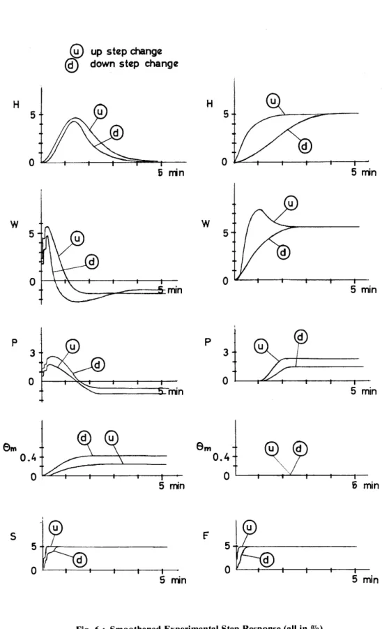
Fig. 6 : Smoothened Experimental Step Response (all in oro)
-15-
--•-•- simutation
- experiment
!z /1 /
5min 5min
- min 5ntn
,
N--••---••db--- min 5min
O O- --- ---- ---
5min 5min
S
5
o
-
---..-v----
/
F 5
o
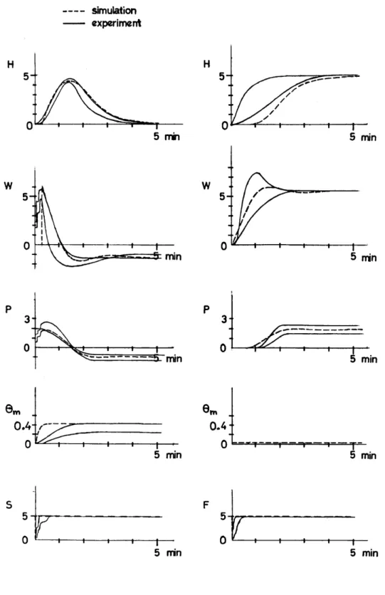
Fig. 7 : Step Responses--Simulation vs. Experiment (in cyo)
4. ANALOG COMPUTER SIMULATION
Analog computer simulation of the mathematical model expressed by Equations (ln) to (10n) is performed as a method of verifying the model and the estimated parameters. To do this, the experimental results in Fig. 2 are smoothened and plotted (Fig. 6) on scales similar to the simulation pen recorder output scales. With the parameter values on Table 2 as starting point, the model is simulated for responses to step changes in feeder speed, F, and screW extruder speed, S, The step responses are observed and compared with the curves on Fig. 6. Parameters (and mathematical model) are adjusted for best fitting of the simulated response curves with the corresponding smoothened experiment curves.
5. 0BSERVATIONS AND ANALYSES
After some preliminary simulations and evaluation, the following observations are deduced : ,a) For an oscillation-free' response of e. to S change, Kei must equal the ratio T4/T2. From the block diagram of the model (Fig. 5), it is clear that the flow Gi can not affect the plastic melt temperature e. directly when Kei- T4/T2 This is true in the physical sense since Gi affects e. only through M2.
b) To maintain a zero response of e. to F change, K. must equal (1-Kei) K2p as
initially calculated on Table 2.
c) The slope of var/S is a linear function of Ki,./Ti.
d) The ratio between the delay element's lag time, L (in milliseconds) and Ti/K. must not be greater than O.6 since Gi oscillates. This and the constraint in c) above fix the values ofL and Ti/Kim•
e) The initial slope of H/S is a linear function of 1/T3.
In the light of the above constraints, analog computer simulation is conducted further and the parameter adjusted until a set of response curves approximated those of the experiment. The values of the parameters giving the satisfactory fitting of curves are :
K2p= 2•5 kg =2•5 K2e= 6. 25 Kps =O.40 Ks =1•16 Kei == O•5 lem=1.25 Kes =O.83 les =2.075 Kim=1.0 Ti=1.43 Kpm=O.60 Kem=O•75 T2 =2.0 T4 =1•O Kis= 1.21 k, =O.90 k, =O.55 K,.=1.0 T, =1.66
These simulation response curves are superimposed on the experiment response curves for com- parison as shown in Fig. 7. While not all of the response curves fit satisfactorily, the results
should be taken considering the following :
1) There is a pair of experiment response curves of the H, W, P and e. variables corres- ponding to `up' and `down' step inputs in both F and S. The difference in the behaviors of the `up' and `down' responses is largely due to the non-linearity character- istics of the system. Furthermore, due to some physical limitations, ideal step changes in Fand S could not be attained in one single step but rather through in- cremental segmented steps as may be seen from the Fand S curves in Fig. 6. I'n both F and S, the `up' step change is closer to the ideal step change. This also accounts for the difference in the `up' and `down' pair of responses of each variable and to the fact that the simulation response curves fit closer to the `up' step change than to the 'down' step change of the experiment (see Fig. 7).
2) The simulation so far conducted has been focused on the curve fitting of H response to S change and of e. response to F change. It may be verified from Fig. 7 that the latter is attained perfectly with em/F=O. H/S fitting is very good except for the
-17-
initial part of the response, This may be improved by modifying that portion of the model affecting H to include a second or higher order lag circuit in place of a first order lag of the present model.
3) The rest of the response curves exhibit varying degree of fitting with the experiment curves and these will be the focus of further study of this process. With a more refined energy balance and in-depth analysis of the temperature distribution in the extruder, it is hoped to achieve an improved fitting of response curves specifically for em/S,P/S and P/F.
5. CONCLUSION
The above modeling and simulation of a plastic extruder shows that, to a certain degree, the model constructed approximates the actual system satisfqctorily within the limits of the trends of responses of the process. The study revealed that with a simple linear model with one time lag element, a good approximation can be attained. However, because of the inherent non-linearity of the system, a set of parameter values can produce desired responses for only unidirectional step input. It is interesting to note further that the values of some time constants and parameters agree very closely with the actual system parameters in the physical sense. A more in-depth investigation of the extruder temperature distribution and energy balance is hoped to yield a better model and improved responses.
REFERENCES
(1) Campbell, D. P., Process Dynamics, John Wiley & Sons, New York, 1958
(2) Hougen, O. A., Watson, K. M., Ragatz, R. A., Chemical Process Principles Part I, John Wiley & Sons, New York, 1954