JAIST Repository https://dspace.jaist.ac.jp/

(1)

Japan Advanced Institute of Science and Technology

JAIST Repository

https://dspace.jaist.ac.jp/

Title 証明数を用いたゲーム木探索の新たなパラダイム

Author(s) 張, 嵩

Citation

Issue Date 2019‑06

Type Thesis or Dissertation Text version ETD

URL http://hdl.handle.net/10119/16064 Rights

Description Supervisor：飯田弘之, 先端科学技術研究科, 博士

(2)

Doctoral Dissertation

A New Paradigm of Game Tree Search Using Proof Numbers

by Zhang Song

Supervisor: Professor Dr. Hiroyuki Iida

Graduate School of Advanced Science and Technology Japan Advanced Institute of Science and Technology

Information Science

June, 2019

(3)

Supervised by

Prof.Dr.Hiroyuki Iida

Reviewed by

Prof. Shun-Chin Hsu Prof.Dr.Tsan-Sheng Hsu Dr.Kiyoaki Shirai

Dr.Minh Le Nguyen Dr.Kokolo Ikeda

(4)

Abstract

Conspiracy number and proof number are two game-independent heuristics in a game- tree search. The conspiracy number is proposed in Conspiracy Number Search (CNS) which is a MIN/MAX tree search algorithm, trying to guarantee the accuracy of the MIN/MAX value of a root node. It shows the scale of “stability” of the root value.

The proof number is inspired by the concept of conspiracy number, and applied in an AND/OR tree to show the scale of “difficulty” for proving a node. It is first proposed in Proof-Number Search (PN-search) which is one of the most powerful algorithms for solving games and complex endgame positions. The Monte-Carlo evaluation is another promising domain-independent heuristic which focuses on the analysis based on random sampling of the search space. The Monte-Carlo evaluation does not reply on any prior knowledge of human and has made significant achievements in complex games such as Go.

In this thesis, we select the conspiracy number search, the proof number search and the Monte-Carlo tree search as three example search algorithms with domain-independent heuristics to study its relations and differences, and finally propose a new perspective of the game tree search with domain-independent heuristics. The relations and differences of the three search algorithms mentioned can be summarized as follows. The Monte- Carlo tree search uses Monte-Carlo evaluations for the leaf nodes to indicate the most promising node for expansion. In other words, the Monte-Carlo evaluation can be regarded as a detector to obtain the information beneath the leaf nodes to forecast the promising search direction in advance. In contrast, the conspiracy number search and the proof number search tend to use the indicators corresponding to the structure or the shape of the search tree that has already been expanded. Therefore, it can be regarded as forecasting the promising search direction according to the information above the leaf nodes. As a natural induction of such understanding of the game tree search using domain-independent heuristics, we may get some improvements by combining the conspiracy number or the proof number idea with the Monte-Carlo evaluation into a search algorithm, which can be

(5)

considered as a combination of “the information above leaf nodes” and “the information beneath the leaf nodes”.

Our research focuses on applying or refining domain-independent heuristics such as the conspiracy number, the proof number and the Monte-Carlo evaluation to achieve such three purposes: (1) enhancing current search algorithm. For this purpose, we proposed the so-called Deep df-pn search algorithm to improve df-pn which is a depth-first version of PN-search by forcing a deeper search with a parameter. The experiments with Connect6 show a good performance of Deep df-pn. (2) Analyzing and visualizing game progress patterns for better understanding of games and master thinking way, such as showing the analysis of the game progress for learners in Chinese Chess tutorial system.

For this purpose, we proposed the so-called Single Conspiracy Number method for long term position evaluation in Chinese Chess and obtained good results. (3) Studying the relations and differences between the conspiracy number, proof number and the Monte- Carlo evaluation and combining “the information above leaf nodes” and “the information beneath the leaf nodes” to propose a new search algorithm with domain-independent heuristics named probability-based proof number search. A series of experiments show that probability-based proof number search outperforms other famous search algorithms for solving games and endgame positions.

Keyword: combinatorial game, domain-independent heuristic, game solver, Monte- Carlo evaluation, game progress pattern

(6)

Acknowledgments

Firstly, I would like to express my special thanks of gratitude to my supervisor professor Hiroyuki Iida who is not only a outstanding scientist in computer science but also a grand master in Japanese Shogi. Under his supervision, I have obtained so much passion and interest in the study of games and artificial intelligence. During my PhD work, professor Iida not only gave me gold opportunities to communicate with other outstanding professors and researchers in the world, but also supported me a lot in my daily life whenever I had problem. I have learned so much from him, and I appreciate him so much.

Secondly, thanks professor Jaap ven den Herik who hosted me in Leiden University for my minor research and helped me so much on our research papers. Also thanks Matej Gruid and Victor Allis who encouraged me and gave me a lot of good advice on my research when I was in Leiden University.

Thirdly, thanks professor Kokolo Ikeda and secretary Setsuko Asakura for the kind help to my study and daily life in Iida lab. Thanks the committee members of my PhD defense: professor Tsan-Sheng Hsu, professor Kiyoaki Shirai and professor Minh Le Nguyen for their excellent work. Also thanks my postgraduate supervisor professor Deng Ansheng for his invitations to Dalian Maritime University. Thanks all the students in Iida lab: Mr Zuo Long, Dr Xiong Shuo, Mr Zhai He, Mr Ye Aoshuang and so on. Thanks all the staff of JAIST.

Next, I will thank my parents who gave me good education and great support in my life. They not only raised me up but also taught me how to be a better man. I love them.

Special Thanks to Ms Xue Yawen, my girl friend. She came to JAIST two years before me and waited for me until I enrolled. Without her, I would not start my PhD study and enjoy my life so much. She is the source of my confidence, courage and happiness. Thank you so much. You are my forever lover, best friend and soul mate. I love you.

Finally, thanks China Scholarship Council for the financial support of my PhD work.

(7)

Today is not easy. Tomorrow may be more difficult. But the day after tomorrow will be fantastic. Keep going and enjoy!

(8)

List of Figures

2-1 An example of MIN/MAX tree [40] . . . 11 2-2 An example of conspiracy numbers (the left column of the number list of

a node is the evaluation value, and the right column of the number list of a node is its corresponded conspiracy number) [40] . . . 12 2-3 An example of the expansion and updating process in the conspiracy num-

ber search (the left column of the number list of a node is the evaluation value, and the right column of the number list of a node is its corresponded conspiracy number) [40] . . . 13 2-4 An example of the seesaw effect: (a) An example game tree (b) Expanding

the most-proving node [19] . . . 17 2-5 An example of a suitable tree for an Othello end-game position. This game

tree has a uniform depth of 4, and the terminal nodes are reached at game end. [19] . . . 18 2-6 The variation in Othello: The number of # of Iterations and # of Nodes.

R = 1.0 is PN-search, R = 0.0 is depth-first search, and 1.0> R > 0.0 is DeepPN. Lower is better. [19] . . . 23 2-7 The reduction rate in Othello: The number of # of Iterations and # of

Nodes. R= 1.0is PN-search, R= 0.0is depth-first search, and1.0> R >

0.0is DeepPN. Lower is better. [19] . . . 24 2-8 # of Iterations in Othello: The changes of Reducing and Increasing Cases

for # of Iterations and # of Nodes [19] . . . 25 2-9 # of Nodes in Othello: The changes of Reducing and Increasing Cases for

# of Iterations and # of Nodes [19] . . . 26

(12)

2-10 The variation in Hex: The changes of Reducing and Increasing Cases for

# of Iterations and # of Nodes [19] . . . 27 2-11 The reduction rate in Hex: # of Iterations and # of Nodes for Hex(4).

R = 1.0 is PN-search, R = 0.0 is depth-first search, and 1.0> R > 0.0 is DeepPN. Lower is better. [19] . . . 27 2-12 Hex: The detail of Fig 2-11. This figure is zoomed 1.0 ≤ R ≤ 0.9. The

lower is better. [19] . . . 28 2-13 One iteration of the general MCTS approach [7] . . . 31 3-1 Relationship between PN-search, df-pn, DeepPN and Deep df-pn . . . 39 3-2 An example of the seesaw effect: (a) An example game tree (b) Expanding

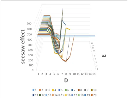
the most-proving node [19] . . . 41 3-3 An example of (a) relevance zone Z and (b) relevance zone Z^′ [55] . . . 43 3-4 Example position 1 of Connect6 (Black is to move and Black wins) . . . . 45 3-5 Example position 2 of Connect6 (Black is to move and Black wins) . . . . 45 3-6 Deep df-pn and df-pn compared in node number (including repeatedly

traversed nodes) with various values of parameter E and D for position 1 (Df-pn when D= 1) . . . 46 3-7 Deep df-pn and df-pn compared in seesaw effect number with various values

of parameter E and D for position 1 (Df-pn when D= 1) . . . 46 3-8 Deep df-pn and df-pn compared in node number (including repeatedly

traversed nodes) with various values of parameter E and D for position 2 (Df-pn when D= 1) . . . 47 3-9 Deep df-pn and df-pn compared in seesaw effect number with various values

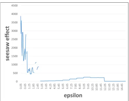
of parameter E and D for position 2 (Df-pn when D= 1) . . . 47 3-10 Node number (including repeatedly traversed nodes) of 1 +ϵ trick with

various values of parameter ϵ for position 1 . . . 51 3-11 Seesaw effect number of 1 +ϵ trick with various values of parameter ϵ for

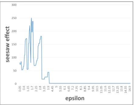
position 1 . . . 52 3-12 Node number (including repeatedly traversed nodes) of 1 +ϵ trick with

various values of parameter ϵ for position 2 . . . 52

(13)

3-13 Seesaw effect number of 1 +ϵ trick with various values of parameter ϵ for position 2 . . . 53 4-1 An example of tactical position where Red is to move (Red wins) . . . 61 4-2 Red’s MIN/MAX value and SCN in positionP₀ with different search depth

(T = 600) . . . 62 4-3 Black’s MIN/MAX value and SCN in position P₁ with different search

depth (T = 600) . . . 62 4-4 Histogram of RSCN_red and RSCN_black (T = 600) . . . 65 4-5 Histogram of V lred and V lblack . . . 65 4-6 Histogram ofRSCN in winning positions, losing positions and drawn po-

sitions (T = 600) . . . 67 4-7 Histogram of V l in winning positions, losing positions and drawn positions 67 4-8 Relationship between high possibility, low possibility and normal possi-

bility of changing the MIN/MAX values of positions not less than the threshold T in advance of the opponent scaled by RSCN . . . 67 4-9 RSCNs for different handicap openings with T = 200 . . . 68 4-10 RSCNs for different handicap openings with T = 600 . . . 68 5-1 Two examples of updating PN by MIN rule in MCPN-search (the square

represents the OR node). . . 77 5-2 Two examples of updating PPN by OR rule in PPN-search (the square

represents the OR node). Notice that PPN = 1 − PN. . . 78 5-3 Two examples of updating PN by SUM rule in MCPN-search (the circle

represents the AND node). . . 78 5-4 Two examples of updating PPN by AND rule in PPN-search (the circle

represents the AND node). Notice that PPN = 1 − PN. . . 79 5-5 Two examples of updating simulation values by taking the average in the

UCT solver or the pure MCTS solver (the square represents the OR node). 82 5-6 Two examples of updating PPN by OR rule in PPN-search (the square

represents the OR node). . . 82 5-7 Comparison of average search time for a P-game tree with 2 branches and

20 layers. . . 84

(14)

5-8 Comparison of average numbers of iterations for a P-game tree with 2 branches and 20 layers. . . 85 5-9 Comparison of the error rate of selected moves for each iteration on P-game

trees with 2 branches and 20 layers. . . 85 5-10 Comparison of average search time for a P-game tree with 8 branches and

8 layers. . . 86 5-11 Comparison of average numbers of iterations for a P-game tree with 8

branches and 8 layers. . . 86 5-12 Comparison of the error rate of selected moves for each iteration on P-game

trees with 8 branches and 8 layers. . . 87 6-1 Example position 3 of Connect6 (Black is to move and Black wins) . . . . 90 6-2 Example position 4 of Connect6 (Black is to move and Black wins) . . . . 90 6-3 Example position 5 of Connect6 (Black is to move and Black wins) . . . . 91 6-4 Example position 6 of Connect6 (Black is to move and Black wins) . . . . 91 6-5 Example position 7 of Connect6 (White is to move and White wins) . . . . 91 6-6 Example position 8 of Connect6 (White is to move and White wins) . . . . 91

(15)

List of Tables

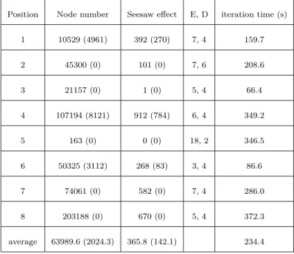
3.1 Different behaviors by changing parameters . . . 42 3.2 Deep df-pn and 1 +ϵ trick compared in the best case (The number in the

bracket represents the reduction percentage compared with df-pn) . . . 53 3.3 Experimental data of Deep df-pn using hill-climbing method (The number

in the bracket represents the difference between Deep df-pn using hill- climbing method and Deep df-pn in the best case) . . . 54

(16)

Chapter 1 Introduction

1.1 Background

Games are classified by the following properties: (1) Zero-sum: Whether the reward to all players sums to zero (in the two-player case, whether players are in strict competition with each other). (2) Information: Whether the state of the game is fully or partially observable to the players. (3) Determinism: Whether chance factors play a part (also known as completeness, i.e. uncertainty over rewards). (4) Sequential: Whether actions are applied sequentially or simultaneously. (5) Discrete: Whether actions are discrete or applied in real-time [7]. Games that are zero-sum, perfect information, deterministic, discrete and sequential are described as combinatorial games. Combinatorial games [5] includes one-player combinatorial puzzles such as Sudoku [31] [17], and no-player automata, such as Conway’s Game of Life [16], but largely confined to two-player games that have a position in which the players take turns changing in defined ways or moves to achieve a defined winning condition, such as chess [22], checkers [42], and Go [33]. Combinatorial games are of interest in artificial intelligence, particularly for automated planning and scheduling [14]. By refining practical search algorithms such as the alpha–beta pruning search [27], we can implement a strong AI in such type of games. Many studies [39]

[27] [43] show that based on such search framework, the strength of AI highly depends on the quality of the heuristic. To obtain reliable heuristic information of games, one possible way is to use expert’s knowledge, usually in the form of scoring game positions.

We call such heuristic as domain-dependent heuristic, because such heuristic is limited

(17)

to work on a certain game and hard to be generalized into other domains. Sometimes, domain-dependent heuristics are not reliable and even cannot be obtained especially in some complex games such as Go. In such case, the domain-independent heuristic is more advanced as it is obtained automatically in a more general way. In this thesis, we will review three typical domain-independent heuristics: Monte-Carlo evaluation [12], conspiracy number [32] and proof number [2]. We discuss the connections and differences of these heuristics in order to give a new perspective of the game tree search with domain- independent heuristics. Based on such new perspective, several enhancements on the search algorithms corresponding to the domain-independent heuristics are achieved, and new applications of the domain-independent heuristics are proposed. Finally, the ultimate purpose is to combine the advantages of these domain-independent heuristics and propose a new advanced search algorithm: probability-based proof number search. We conduct experiments to evaluate the performance of the probability-based proof number search and obtain significant results in the end. The success of probability-based proof number search not only makes breakthrough in real applications, but also theoretically proves our understanding on the new perspective of game tree search in this thesis.

Starting from Deep Blue [9] defeating the Chess world champion in 1997, search algorithms in combinatorial games have been significantly developed from a brute-force large-scale search [30] to a very selective heuristic search. The search efficiency is significantly improved by both using the high-quality domain-dependent heuristic and extremely cutting off of the brunches of the game tree. While after AlphaGo [44] defeating the Go world champion in 2017, a new generation of the game tree search has been started. The Monte-Carlo tree search (MCTS) and its variants based on domain-independent sampling and simulations become more and more successful than other conventional approaches.

The focus of Monte Carlo tree search is on the analysis of the most promising moves, expanding the search tree based on random sampling of the search space. The application of Monte-Carlo tree search in games is based on many playouts. In each playout, the game is played out to the very end by selecting moves at random. The final game result of each playout is then used to weight the nodes in the game tree so that better nodes are more likely to be chosen in future playouts. Different from the domain-dependent heuristic, such playout does not reply on any prior knowledge of human. Using such

(18)

domain-independent heuristic in a search algorithm combined with large-scale parallel computing and deep neural network, computer can master different games beyond human experts [46] [45]. In other words, the success of Monte-Carlo tree search in Go can be considered to be a success of domain-independent heuristics in the game tree search.

In fact, before Monte-Carlo tree search, there have been some successful game tree search algorithms using the domain-independent heuristics, such as conspiracy number search (CNS) [32] and proof number search (PN-search) [2]. The core idea of conspiracy number search is using a vector of conspiracy numbers to indicate the likelihood of the root taking on a particular value. More precisely, the conspiracy number is the minimum number of leaf nodes in the tree that must change their score (by being searched deeper) to result in the root taking on that new value [52]. For each iteration in the search process, the conspiracy number search always expands the most promising nodes indicated by the conspiracy numbers to make the game tree grow from an “unstable” state to a

“stable” state in an expectantly fastest way. Different from the Monte-Carlo tree search, the conspiracy number search can be considered to be a search algorithm using both the domain-dependent heuristic (the scores of leaf nodes) and the domain-independent heuristic (the conspiracy number). Moreover, the conspiracy number is obtained, not based on the sampling or the simulations of the game, but based on the structure or the shape of a game tree that has already been expanded. The conspiracy number evaluates the

“stability” of the root score, indicating a proper ending state of a search. Such theoretical concept is very promising, but suffers from a low efficiency and slow convergence in practical implementations, because it takes too much time and storage to compute and record the vector of conspiracy numbers for each node.

To incorporate the conspiracy number idea into a real application, the proof number search (PN-search) is proposed as a game solver searching on an AND/OR tree. Other than using the vector of conspiracy numbers, PN-search simplifies the conspiracy numbers into two numbers: a proof number (pn) and a disproof number (dn), showing the scale of difficulty in proving and disproving a node, respectively. More precisely, for all unsolved nodes (leaf nodes), the proof number and disproof number are 1. For a winning node, the proof number and disproof number are 0 and infinity, respectively. For a non-winning node, it is the reverse. For internal nodes, the proof number and disproof number are back

(19)

propagated from its children following MIN/SUM rules: at OR nodes, the proof number equals the minimum proof number of its children, and the disproof number equals the summation of the disproof numbers of its children. It is the reverse for AND nodes. For each iteration, going from the root to a leaf node, PN-search selects either the child with the minimum proof number at OR nodes, or the child with the minimum disproof number at AND nodes. Finally, it regards the leaf node arrived at as the most proving node for expansion. Without scoring the game positions, the proof number search completely uses the domain-independent heuristic based on the structure of an AND/OR tree. It becomes one of most successful search algorithms for solving games and endgame positions.

In this thesis, we select the conspiracy number search, the proof number search and the Monte-Carlo tree search as three example search algorithms with domain-independent heuristics to study the relations and the differences between the conspiracy number, the proof number and the Monte-Carlo evaluation. Based on the discussion, we will find a new perspective of the game tree search with domain-independent heuristics. According to the introduction above, the Monte-Carlo tree search uses Monte-Carlo evaluations as domain-independent heuristics for the leaf nodes to indicate the promising search node for expansion. In other words, the Monte-Carlo evaluation can be regarded as a kind of detector to obtain the information beneath the leaf nodes to forecast the promising search direction in advance. In contrast, the conspiracy number and the proof number are indicators based on the structure or the shape of the search tree that has already been expanded. In other words, the conspiracy number and the proof number forecast the promising search direction by using the information above the leaf nodes. As a natural induction of such understanding of game tree search with domain-independent heuristics, there should be potential improvements by combining the conspiracy number or the proof number idea with the Monte-Carlo evaluation in the search algorithm. It can be considered as a combination of using the “information above the leaf nodes” and the “information beneath the leaf nodes”. A typical search algorithm among this category is the Monte-Carlo proof number search, using Monte-Carlo evaluations for the leaf nodes and proof number search rules to expand the search tree. However, the Monte-Carlo proof number search is not a good combination of the Monte-Carlo evaluation and the proof number search, because Monte-Carlo evaluation leads to real numbers but the proof num-

(20)

ber search updating rules are proposed for integer numbers, which causes the information loss. Based on such theoretical consideration, we propose a new search algorithm named probability-based proof number search (PPN-search). We conduct experiments to ver- ify the effectiveness of the probability-based proof number search. Experimental results show that probability-based proof number search outperforms other existing approaches in solving games or endgame positions. The success of probability-based proof number search not only makes breakthrough in real applications, but also theoretically prove our new perspective on the game tree search with domain-independent heuristics.

1.2 Research Questions

Our research focuses on applying and refining domain-independent heuristics, such as the conspiracy number, the proof number and the Monte-Carlo evaluation, to achieve such three goals: (1) Enhancing current search algorithm. For this purpose, we propose the so-called Deep df-pn search algorithm to improve df-pn, an efficient variant of the proof number search by forcing a deeper search with a parameter. It shows a good performance in solving positions of Connect6. (2) Analyzing and visualizing game progress patterns for better understanding of games and master’s thinking way. For this purpose, We propose the so-called single conspiracy number method for long term position evaluations in Chinese Chess and obtain good results. (3) Based on the theory of “the information above the leaf nodes” and “the information beneath the leaf nodes”, we propose a new advanced search algorithm for solving games and endgame positions named probability- based proof number search to improve the efficiency of the original one. We conduct a series of experiments to confirm that the probability-based proof number search is more efficient than other search algorithms for solving games, such as the proof number search, the Monte-Carlo proof number search, the UCT solver and the pure MCTS solver.

1.3 Structure of the Thesis

The dissertation includes 6 chapters: introduction, literature review, Deep df-pn, single conspiracy number, probability-based proof number search, and conclusion. In this dissertation, one grand argument is proposed, then several new findings and further discussions

(21)

are incorporated to support this argument.

Chapter 1. Introduction. We select the conspiracy number search, the proof number search and the Monte-Carlo tree search as three example search algorithms with domain- independent heuristics to introduce the development of game-independent heuristics. Base on the introduction, we propose such argument: conspiracy number and proof number are two game-independent heuristics using “the information above leaf nodes” corresponding to the structure or the shape of the part of the search tree that has already been expanded to indicate the most promising node for expansion, while Monte-Carlo tree search method

“the information beneath the leaf nodes” obtained by simulations to indicate the most promising node for expansion. There are high similarity and closed connection between the conspiracy number, the proof number and the Monte-Carlo evaluation. Therefore, we could get potential improvements by combining the conspiracy number or the proof number idea with Monte-Carlo evaluation. This can be regarded as the combination of

‘the information above leaf nodes” and “the information beneath the leaf nodes”.

Chapter 2. Literature Review. In this chapter, we introduce related works before our study. We classify the game-independent heuristics into three categories: “using the information above the leaf nodes”, “using the information beneath the leaf nodes”

and “combining the information above and beneath the leaf nodes”. The “using the information above the leaf nodes” category includes the conspiracy number search, the proof number search, df-pn and Deep proof number search. The “using the information beneath the leaf nodes” category includes the Monte-Carlo tree search and the Monte- Carlo tree search solver which is a variant of Monte-Carlo tree search for solving endgame positions. The “combining the information above and beneath the leaf nodes” includes the Monte-Carlo proof number search which is a variant of proof number search combining with Monte-Carlo evaluations.

Chapter 3. Deep df-pn. Depth-first proof-number search (df-pn) is a powerful variant of proof number search algorithms, widely used for AND/OR tree search or solving games.

However, df-pn suffers from the seesaw effect, which strongly hampers the efficiency in some situations. In this chapter, we propose a new depth-first proof number algorithm called Deep depth-first proof-number search (Deep df-pn) to reduce the seesaw effect in df-pn. The difference between Deep df-pn and df-pn lies in the proof number or

(22)

disproof number of unsolved nodes. It is 1 in df-pn, while it is a function of depth with two parameters in Deep df-pn. By adjusting the value of the parameters, Deep df-pn changes its behavior from searching broadly to searching deeply. The chapter shows that the adjustment is able to reduce the seesaw effect convincingly. For evaluating the performance of Deep df-pn in the domain of Connect6, we implemented a relevance-zone- oriented Deep df-pn that worked quite efficiently. The experimental results indicate that improving efficiency by the same adjustment technique is also possible in other domains.

Chapter 4. Single Conspiracy Number. Single Conspiracy Number (SCN) is a variant concept of conspiracy number and proof number which indicates the difficulty of a root node changing its MIN/MAX value to a certain score. It makes up the drawbacks of conspiracy number on computing complexity and storage cost, which can be easily applied into different search frameworks. This chapter explores the potential usage of SCN as a long-term position evaluation to understand in-depth game progress patterns.

Chinese Chess is chosen as a test bed for this study, whereas a strong open source AI engine ‘Xiangqi Wizard’ is used. It is implemented with alpha-beta search and modified to produce SCNs during the search process. Experiments are conducted on different types of positions including tactical positions, drawn positions and opening positions. The experimental results show that SCN is more consistent and accurate for long-term position evaluation than the conventional way using evaluation function values only. One application of SCN is the Chess tutorial system. Besides the evaluation function, SCN provides another scalar axis showing the changes of the game progress. It helps the users obtain more information about the game. Using SCN together with evaluation function values enables us to better understand game progress patterns.

Chapter 5. Probability-based Proof Number Search. Probability-based proof number search (PPN-search) is a game tree search algorithm improved from proof number search (PN-search) [2], with applications in solving games or endgame positions. PPN- search uses one indicator named “probability-based proof number” (PPN) to indicate the

“probability” of proving a node. The PPN of a leaf node is derived from Monte-Carlo evaluations. The PPN of an internal node is back propagated from its children following AND/OR probability rules. For each iteration, PPN-search selects the child with the maximum PPN at OR nodes and minimum PPN at AND nodes. This holds from the

(23)

root to a leaf. The resultant node is considered to be the most proving node for expansion. In this chapter, we investigate the performance of PPN-search on P-game trees [28] and compare our results with those from other game solvers such as MCPN-search [38], PN-search, UCT solver, and the pure MCTS solver [54]. The experimental results show that (1) PPN-search takes less time and fewer iterations to converge to the correct solution on average, and (2) the error rate of selecting a correct solution decreases faster and more smoothly as the iteration number increases.

Chapter 6. Conclusion and Future Works. We summarize all the introductions and discussions above, and make a conclusion. In addition, several possible future works are presented.

(24)

Chapter 2 Literature Review

In this chapter, we introduce related works before our study. We classify the game- independent heuristics into three categories: “using the information above the leaf nodes”,

“using the information beneath the leaf nodes” and “combining the information above and beneath the leaf nodes”. The “using the information above the leaf nodes” category stands for the class of search algorithms using domain-independent heuristics based on the structure or the shape of the search tree that has already been expanded, including the conspiracy number search, the proof number search, df-pn and Deep proof number search.

“using the information beneath the leaf nodes” category stands for the class of search algorithms using domain-independent heuristics based on the Monte-Carlo evaluation, including the Monte-Carlo tree search and the Monte-Carlo tree search solver. For the

“combining the information above and beneath the leaf nodes”, we introduce a typical approach: the Monte-Carlo proof number search as a benchmark.

2.1 Using the Information above the Leaf Nodes

2.1.1 Introduction

In this section, we select the conspiracy number search, the proof number search and its variants as example search algorithms with domain-independent heuristics using the information above the leaf nodes. All the mentioned search algorithms use the conspiracy number or the proof number as a kind of indicators based on the structure or the shape of the search tree that has already been expanded. In other words, the conspiracy number

(25)

and the proof number forecast the promising search direction by using the information above the leaf nodes. Here, We also introduce the seesaw effect that highly hampers the efficiency of the original proof number search. Then the Deep proof number search is introduced to solve this problem.

2.1.2 Conspiracy Number Search

Conspiracy Number Search (CNS) [32] is a MIN/MAX tree search algorithm, trying to guarantee the accuracy of the MIN/MAX value of a root node. The likelihood of the root taking on a particular value is reflected in that value’s associated conspiracy number. The conspiracy number is the minimum number of leaf nodes in the tree that must change their score (by being searched deeper) to result in the root taking on that new value [41].

The tree is grown in a way that restricts the set of likely root values. The formalism of the conspiracy number is given below [41].

Whennis a leaf node, if the evaluation ofnisv, then the conspiracy number associated withv is 0 and for all other values is 1. If that leaf node is terminal (its value is absolute), then the alternative values can be viewed as requiring ∞ conspirators.

When n is an internal node, consider breaking the set of conspiracy numbers into two groups: the numbers required to increase a node’s value (↑needed) and those to decrease it (↓needed). Values below the MIN/MAX score in ↑needed and above the MIN/MAX score in ↓ needed are assigned 0. ↑ needed and ↓ needed of an interior node’s children can be combined to form the parent’s conspiracy numbers,CN, using the following rules (with v being a value andm being the MIN/MAX value):

(a) If v =m,

CN(v) = 0.

(b) For a MAX node:

CN(v) = ∑ all children i

↓needed_i(v), for all v < m.

CN(v) = M in all children i

↑neededi(v), for all v > m.

(26)

(c) For a MIN node:

CN(v) = M in all children i

↓neededi(v), for all v < m.

CN(v) = ∑ all children i

↑needed_i(v), for all v > m.

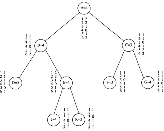
Fig. 2-1, Fig. 2-2 and Fig. 2-3 show an example of computing, expansion and updating conspiracy numbers for a MIN/MAX tree. For each iteration, the conspiracy number search always selects the leaf node corresponding to the minimum conspiracy number of the root to eliminate the unstable element in the tree. The conspiracy number is a very promising concept of the domain-independent heuristic, but suffers from a low efficiency in real applications. There are mainly two reasons: (1) it takes too much time and storage to compute and record the conspiracy numbers (2) the algorithm converges slowly, sometimes even cannot converge. As a result, the conspiracy number becomes a good theoretical benchmark to be improved.

Figure 2-1: An example of MIN/MAX tree [40]

2.1.3 Proof Number Search

To incorporate the conspiracy number idea into a real application, the proof number search (PN-search) is proposed as a game solver searching on an AND/OR tree. Proof- Number Search (PN-search) [2] is a native best-first algorithm, using proof numbers and disproof numbers, always expanding one of the most-proving nodes. All nodes have proof and disproof numbers, they are stored to indicate which frontier node will be expanded, and updated after expanding. A proof (disproof) number shows the scale of difficulty in

(27)

Figure 2-2: An example of conspiracy numbers (the left column of the number list of a node is the evaluation value, and the right column of the number list of a node is its corresponded conspiracy number) [40]

proving (disproving) a node. The expanded node is called the most-proving node, which is the most efficient one for proving (disproving) the root. By exploiting the search procedure, two characteristics of the search tree are established [50]: (1) the shape (determined by the branching factor of every internal node), and (2) the values of the leaves (in the end they deliver the game theoretic value). Basically, unenhanced PN-Search is an unin- formed search method that does not require any game-specific knowledge beyond its rules [25]. The formalism is given below.

Letn.pnandn.dnbe the proof number and disproof number of a noden, respectively.

When n is a terminal node (a) If n is a win for the attacker:

n.pn= 0 n.dn=∞ (b) If n is a loss for the attacker:

n.pn=∞ n.dn= 0

(28)

Figure 2-3: An example of the expansion and updating process in the conspiracy number search (the left column of the number list of a node is the evaluation value, and the right column of the number list of a node is its corresponded conspiracy number) [40]

(c) If the value ofn is unknown:

n.pn= 1 n.dn= 1 When n is an internal node

(a) If n is an OR node:

n.pn= M in

nc∈children of nn_c.pn

n.dn= ∑

nc∈children of n

n_c.dn (b) Whenn is an AND node

(29)

n.pn= ∑

nc∈children of n

n_c.pn

n.dn= M in

nc∈children of nnc.dn

A most-proving node is a leaf node that is selected by tracing nodes from the root node in the following way.

• For each OR node, trace the child with the minimum proof number.

• For each AND node, trace the child with the minimum disproof number.

Note that Allis et al. [2] defined the most-proving node as the left-most one, if there is arbitrariness.

2.1.4 Df-pn

Although PN-search is an ideal AND/OR-tree search algorithm, it still has at least two problems. We mention two of them. The first one is that PN-search uses a large amount of memory space because it is a best-first algorithm. The second one is that the algorithm is not efficient as hoped for because of the frequently updating of the proof and disproof numbers. To solve the problems, Nagai [34] proposed a depth-first like algorithm using both proof number and disproof number. He called it df-pn (depth-first proof-number search). The procedure of df-pn can be characterized as (1) selecting the most-proving node, (2) updating the thresholds of proof number or disproof number in a transposition table, and (3) applying multiple iterative deepening until the ending condition is satisfied.

Although df-pn is a depth-first like search, it has a same behavior as PN-search. The equivalence between PN-search and df-pn is proved in [34].

In df-pn, proof number and disproof number are renamed as follows.

n.ϕ=



 n.pn

(

n is an OR node ) n.dn

(

n is an AND node )

n.δ =



 n.dn

(

n is an OR node ) n.pn

(

n is an AND node )

(30)

Moreover, each node n has two thresholds: one for the proof number thpn and the other for the disproof numberth_dn. Similarly, th_pn and th_dn are renamed as follows.

n.thϕ=





n.th_pn (

n is an OR node ) n.th_dn

(

n is an AND node )

n.thδ=





n.th_dn (

n is an OR node ) n.th_pn

(

n is an AND node )

Df-pn expands the same frontier node as PN-search in a depth-first manner guided by a pair of thresholds (thpn, thdn), which indicates whether the most-proving node exists in the current subtree [21]. The procedure is described below [34].

Procedure Df-pn

For the root node r, assign values for r.thϕ and r.thδ as follows.

r.th_ϕ=∞ r.th_δ =∞

Step 1. At each node n, the search process continues to search below n until n.ϕ≥ n.th_ϕ orn.δ ≥n.th_δ is satisfied (we call it ending condition).

Step 2. At each node n, select the child n_c with minimum δ and the child n₂ with second minimum δ. (If there is another child with minimumδ, that isn₂.) Search below n_c with assigning

n_c.th_ϕ=n.th_δ+n_c.ϕ−∑

n_child.ϕ n_c.th_δ = min (n.th_ϕ, n₂.δ+ 1) Repeat this process until the ending condition holds.

Step 3. If the ending condition is satisfied, the search process returns to the parent node ofn. If n is the root node, then the search is totally over.

(31)

2.1.5 The Seesaw Effect

PN-search and df-pn are highly efficient in solving games. However, both are facing the drawback named as seesaw effect [18]. It can be best characterized as frequently going back to the ancestor nodes for selecting the most-proving node. Pawlewicz and Lew [36], and Kishimoto et al. [26] [24] showed one such weak point of df-pn. The weak point has been named the seesaw effect by Hashimoto [18].

To explain it precisely, we show, in Fig. 2-4, an example where the root node has two subtrees. The size of both subtrees is almost the same. Assume that the proof number of subtree L is larger than the proof number of subtree R. In this case, PN-search or df-pn will continue search in subtree R, which means that the most-proving node is in subtree R. After PN-search or df-pn has expanded the most-proving node, the shape of the game tree will change as shown in Fig. 2-4(b). By expanding the most-proving node, the proof number of subtree R becomes larger than the proof number of subtree L. So PN-search or df-pn changes its searching direction from subtree R to subtree L. In turn, when the search expands the most-proving node in subtree L, then the proof number of subtree L becomes larger than the one in subtree R. Thus, the search changes its focus from subtree L to subtreeR. This change keeps going back and forth, which looks like a seesaw. Therefore, it is named as seesaw effect.

The seesaw effect happens when the two trees are almost equal in size. If the seesaw effect occurs frequently, the performance of PN-search and df-pn deteriorates significantly and cannot reach the required search depth. In games which need to reach a large fixed search depth, the seesaw effect works strongly against efficiency.

The seesaw effect is mostly caused by two issues: the shape of game tree and the way of searching. Concerning the shape of game tree, there are two characteristics: (1) a tendency of the newly generated children to keep the size equal and (2) the fact that many nodes with equal values exist deep down in a game tree. If the structure of each node remains almost the same (cf. characteristic 1), then the seesaw effect may occur easily. For characteristic 2, it is common in games such as Othello and Hex to search a large fixed number of moves before settling. This is also the case in connect-type games such as Gomoku and Connect6 which have a sudden death in the game tree. Therefore, it is necessary to design a new search algorithm to reduce the seesaw effect in these games.

(32)

PN = 999 PN = 1000

L R L R

Most-Proving Node

PN = 1001 PN = 1000

(a) (b)

Figure 2-4: An example of the seesaw effect: (a) An example game tree (b) Expanding the most-proving node [19]

2.1.6 Deep Proof Number Search

This section is updated and abridged from the following publication.

• Ishitobi, T. (2016). Deep Proof-Number Search and Aesthetics of Mating Problems.

JAIST Press.

In this section, we introduce a new search algorithm based on proof numbers named Deep Proof-Number Search (DeepPN). DeepPN is a variant of the original PN-search.

Each node in the search tree has two indicators: the proof number and the disproof number. Additionally, for DeepPN, each node is assigned a so-called deep value. The deep values are determined and updated by the terminal node analogously to the proof and disproof numbers. DeepPN has been designed to: (1) combine the best-first and the depth-first search, and (2) to try and solve the problem of the seesaw effect. For evaluating the performance of DeepPN, we use endgame positions of Othello and Hex.

The Basic Idea of DeepPN

In the original PN-search, the most-proving node is defined as follows [2].

Definition 1. For any AND/OR tree T, a most-proving node of T is a frontier node of T, which by obtaining the value true reduces T’s proof number by 1, while by obtaining the value false reduces T’s disproof number by 1.

This definition implies that the most-proving node sometimes exists in a plural form in a tree, i.e., there are many fully equivalent most-proving nodes. For example, if the

(33)

OR node AND node Game End

2,3 2,1

1,1 1,1

2,2 2,2

2,1 2,1

1,1 1,1 1,1 1,1

Figure 2-5: An example of a suitable tree for an Othello end-game position. This game tree has a uniform depth of 4, and the terminal nodes are reached at game end. [19]

child nodes have the same proof or disproof number then both subtrees have each a most- proving node. The situation that the child nodes has the same proof (disproof) number in an OR (AND) node is called a tie-break situation. Now, we have the question about which most-proving node is the best for calculating the game-theoretical value. PN-search chooses the leftmost node with the smallest proof (disproof) number, also in a tie-break situation. In particular, the proof and disproof number do not take other information into account, and therefore PN-search cannot choose a more favorable most-proving node in a tie-break situation.

Determining the best most-proving node in a tie-break situation is a difficult task, because the answer depends on many aspects of the game. However, when focusing on games which build up a suitable tree, we may develop some solutions. In a suitable tree, the “best” most-proving node is indicated by its depth number. See the example given in Fig 2-5.

This game tree is from the Othello [8]. The end of the game is shown by “Game End”

in Fig 2-5. All level-two nodes are most-proving nodes, because the proof numbers of child nodes under the root node are the same (i.e., 2). So, we have a tie-break situation.

Now, in the next search step, PN-search will focus on the most-proving node that exists in left side as produced by the original PN-search algorithm. However, if the search focuses

(34)

immediately on the most-proving node of the right side, then the search will be more efficient, because the nodes on the left side do not reach the game end and their value cannot be found yet. In contrast, nodes that exist at the right side reach the game end, and if we try to expand these nodes, then the game value of each node is known. In this example, we follow the idea that a most-proving node in the deepest tree of a suitable game tree, is the best.

To test this idea, we performed a small experiment. We prepared an original PN- search and a modified PN-search. In a tie-break situation, PN-search focuses on a most- proving node that exists in the leftmost node, and the modified PN-search focuses on the deepest most-proving node. For checking performance, we prepared 100 Othello endgame positions. The performance of the modified PN-search is better than the results of the original PN-search (about 10% reduction). These results suggest that the deepest most- proving node works advantageously for finding the game-theoretical value.

In addition, the example of Fig 2-5 shows the essence of the seesaw effect. If the game end exists and has a depth of more than 4, then the search for a proof number goes back and forth between the two subtrees. Even if the game end is of depth 4, then the search that focuses on the right subtree will change its focus on the left subtree. But, when modifying PN-search, the small seesaw effect is suppressed. This phenomenon of modifying PN-search suggests a new heuristic. The search depth of nodes can be used for solving the seesaw effect in a suitable game tree. In fact, this is what 1 + ϵ trick [36]

in effect tries to accomplish, to stay deep in a suitable game tree. For more detail of 1 + ϵ trick, see section 3.3.4 in chapter 3. Now, let us try to think of a new technique.

For instance, consider the moves that the modified PN-search plays when finding the deepest most proving node. We noticed that these moves combined best-first with depth- first behavior. The modified PN-search works in a best-first manner, and in a tie-break situation, PN-search work depth-first for the most-proving nodes. Depending on how often tie-breaks occur, the algorithm works more frequently best-first than depth-first.

The resulting improvement, when measured in number of iterations and nodes leads to a small result. Thus, we will design a new algorithm that can change the ratio of best-first manner and depth-first manner. Its description is an follows. This system is named Deep Proof-Number Search (DeepPN). Here,n.ϕmeans proof number in OR node and disproof

(35)

number in AND node. In contrast, n.δ means proof number in AND node and disproof number in OR node.

1. The proof number and disproof number of node n are now calculated as follows.

n.ϕ =





n.pn (n is an OR node) n.dn (n is an AND node) n.δ =





n.dn (n is an OR node) n.pn (n is an AND node) 2. When n is a terminal node

(a) When n is proved (disproved) and n is an OR (AND) node, i.e., OR wins

n.ϕ= 0 n.δ =∞

(b) When n is disproved (proved) and n is an AND (OR) node, i.e., OR does not win

n.ϕ=∞, n.δ = 0 (c) When n is unsolved, i.e., its value is unknown

n.ϕ= 1, n.δ = 1

(d) When n is terminal node, then n has deep value

n.deep= 1

n.depth (2.1)

3. When n is an internal node

(36)

(a) The proof and disproof number are defined as follows

n.ϕ = min

nc∈children of nn_c.δ

n.δ = ∑

nc∈children of n

n_c.ϕ

(b) The deep values, DPN(n) and n.deep are defined as follows.

n.deep = n_c.deep where n_c= arg min

ni∈unsolved children

DP N(n_i) (2.2) DP N(n) = (1− 1

n.δ+ 1)R+n.deep(1−R) (0.0≤R ≤1.0) (2.3) The proof and disproof number are the same as in the original PN-search. The improvement is the new term, i.e., the concept of the deep value. The deep value in a terminal node is calculated by formula (2.1). The deep value is designed to decrease inversely with depth. In an internal node, calculating the deep value has only a limited complexity. First, we define a function named DPN (see formula 2.3). DPN has two features: (a) n.δ is normalized and designed to become larger according to the growth of n.δ and (b) a fixed parameter R is chosen. R has a value between 0.0 and 1.0. If R is 1.0 then DeepPN works the same as PN-search, and ifR is 0.0 then DeepPN works the same as a primitive depth-first search. Therefore, the normalized δ fulfills the role of best-first guide and the deep acts as a depth-first guide. This means that by changing the value of R, the ratio of best-first and depth-first search of DeepPN can be adjusted. Second, in an internal node, the deep value is updated by its child nodes using formula (2.2). The deep value of node n is decided by a child noden_c which has smallestDP N(n_c). A point to notice is that the updating value is only deep, not DP N(n_c). Additionally, whenn_c is solved, then the deep value of n_c is ignored inarg min.

In DeepPN, an expanding node in each iteration is chosen as follows.

select_expanding_node(n) := arg min

nc∈children of n except solved

DP N(nc) (2.4)

(37)

This sequence is repeated until the terminal node is reached. That terminal node is the node that is to be expanded. IfR = 1.0, then this expanding node is the most-proving node.

Performance with Othello

For measuring the performance of DeepPN, we prepared a solver using the DeepPN algorithm and Othello endgame positions. We configured a primitive DeepPN algorithm for investigating the effect of DeepPN only, without any supportive mechanisms such as transposition tables and ϵ-thresholds. We prepared 1000 Othello endgame positions.

They are constructed as follows. The positions are taken from the 8 x 8 board. We play 44 legal moves at random from the begin position. This implies that 48 squares from the 64 are covered. So, the depth of the full tree to the end is 16.

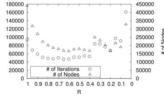
In all our experiments DeepPN is applied to these 1000 endgame positions. Our focus is the behavior of R (see formula (2.3)). For R = 1.0, DeepPN works the same as PN- search and shows the same results. For R = 0.0, DeepPN works the same as a primitive depth-first search. WhenR is between 1.0 to 0.0, then DeepPN behaves as a mix between best-first and depth-first. We changed R from 1.0 to 0.0 by increments of 0.05. We focus on the values of two concepts, viz. the number of iterations and the number of nodes. The number of iterations is given by counting the number of traces of finding the most-proving node from the root node. This value indicates an approximate execution time unaffected by the specifications of a computer. The number of nodes is an indication of the total number of nodes that are expanded by the search. This value is an approximation of the size of memory needed for solving. We show the results in Fig 2-6 and 2-7.

Figure 2-6 shows the variation of (1) the number of iterations and (2) the number of nodes. Each point is as mean value calculated from the results of 1000 Othello endgame positions. R = 1.0 shows the results of PN-search, and this value is the base for comparison. As R goes to 0.8, the number of iterations and nodes decrease almost by half.

From R= 0.8to0.6, the number of iterations stops decreasing, but the number of nodes decreases slowly. From R = 0.6 to 0.4, the decrease stops, and the number of iterations starts increasing again slowly. In R = 0.35, both numbers increase rapidly. We see that forR of around 0.4, the balance between depth-first and best-first behavior appears to be

(38)

0 20000 40000 60000 80000 100000 120000 140000 160000 180000

0 0.1 0.2 0.3 0.4 0.5 0.6 0.7 0.8 0.9 1

0 50000 100000 150000 200000 250000 300000 350000 400000 450000

# of Iterations # of Nodes

R

# of Iterations

# of Nodes

Figure 2-6: The variation in Othello: The number of # of Iterations and # of Nodes.

R= 1.0is PN-search,R = 0.0 is depth-first search, and1.0> R >0.0 is DeepPN. Lower is better. [19]

optimal. We surmise that DeepPN is stuck in one subtree and cannot get away since the algorithm is too strongly depth-first. For R = 0.35 to 0.2, the number of iterations and nodes is decreasing. Around R = 0.2, the balance was broken again, and is decreasing towards0.1. Finally, DeepPN performs worse whenR approaches0.0closely. In R= 0.0, almost no Othello end game position can be solved, and this value is omitted from Fig 2-6.

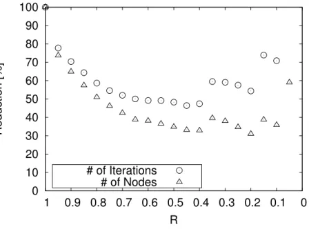
In Figure 2-6, the scale of the number of iterations and nodes are different. To ease our understanding, Figure 2-7 shows the amount of the reduction rate. This reduction rate is normalized by the result of PN-search, i.e., the reduction rate of R = 1.0 is 100%. Each point is the mean value of the reduction rate calculated by the results of 1000 Othello endgame positions. The results of 2-7 show almost the same characteristics as 2-6. There is a different point where the number of iterations decreases afterR= 0.8and the number of nodes decreases afterR = 0.6. In Figure 2-7, the number of iterations decreased about 50% inR = 0.4and the number of nodes decreased about 35% inR = 0.4. Thus, DeepPN reduced the number of iterations (≈ time) to half and the number of nodes (≈ space) to one-third. In R = 0.05, the number of iterations increased to over 100%, which is not shown.

(39)

0 10 20 30 40 50 60 70 80 90 100

0 0.1 0.2 0.3 0.4 0.5 0.6 0.7 0.8 0.9 1

Reduction [%]

R

# of Iterations

# of Nodes

Figure 2-7: The reduction rate in Othello: The number of # of Iterations and # of Nodes.

Finally, we show two graphs about the changes in reducing and increasing cases in Othello endgame positions in Fig 2-8 and 2-9. Please note that in Fig 2-8 and 2-9 we showed the number of iterations and number of nodes.

The plots for reducing cases give the number of Othello endgame positions which are solved efficiently compared to PN-search, i.e., the reduction rate is under 100%. In contrast, the plots for increasing cases give the number of Othello endgame positions that have a reduction rate over 100%. The vertical axis shows the number of Othello endgame positions. Figure 2-8 shows the number of iterations by which the reducing cases decrease slowly from R = 0.95 to 0.4. Likewise, for number of nodes the graph decreases slowly fromR= 0.95to0.4. AroundR= 0.4, the trend is broken, and the number of increasing cases increases rapidly. From R = 0.35 to 0.2 and from 0.15to 0.1, the number of cases does not change much. This result indicates that the reason of decreasing from R= 0.35 to0.2is shown in Fig 2-6 and 2-7. As the number of cases is not changed, the decreasing number of iterations and nodes of the Othello end game positions are caused by reducing cases. In brief, some Othello end positions can be handled efficiently as R is reduced.

But, for some Othello end game positions a changing R causes an increase. Therefore, Othello end game positions can be categorized in relation toR. The first group belongs to

(40)

0 100 200 300 400 500 600 700 800 900 1000

0 0.1 0.2 0.3 0.4 0.5 0.6 0.7 0.8 0.9 1

# of cases

R

# of Reducing Cases

# of Increasing Cases

Figure 2-8: # of Iterations in Othello: The changes of Reducing and Increasing Cases for

# of Iterations and # of Nodes [19]

R= 0.95to0.05. This group does not react to changes in R, they do not switch between the reducing case and increasing case. We can see this group clearly from R = 0.95 to 0.40. The second group belongs to R = 0.35 to 0.2. This group fitted from R = 0.95 to 0.4, and they could not keep efficiency work after R = 0.4. The third group belongs to R = 0.15 to 0.1, and the characteristics of this group are the same as for the second group. In either group, the cases are not efficiently close to R = 0.0.

The question remains when DeepPN works most efficiently in the Othello endgame position for 16-ply. The answer depends on the group of Othello endgame positions.

However, if we have to choose the bestR, then a value of around0.65is a good compromise for most cases.

Performance with Hex

For measuring the performance of DeepPN, we also prepared a solver for Hex [3]. As for the experiments of Othello, we created a primitive DeepPN algorithm for checking the effect of DeepPN only. The Hex program is a simple program that does not have any other mechanisms such as an evaluation function. Our Hex program uses a 4 x 4 board (called Hex(4)), and tries to solve that board using DeepPN. Our focus is on the behavior of R (see formula 2.3). Concerning the characteristics of R, please see section

(41)

0 100 200 300 400 500 600 700 800 900 1000

0 0.1 0.2 0.3 0.4 0.5 0.6 0.7 0.8 0.9 1

# of cases

R

# of Reducing Cases

# of Increasing Cases

Figure 2-9: # of Nodes in Othello: The changes of Reducing and Increasing Cases for # of Iterations and # of Nodes [19]

2.1.6 or 2.1.6. We changed R from 0.0 to 1.0 by 0.5, and tried to solve Hex(4) 10 times in eachR. The legal moves of Hex are sorted randomly in every configuration, viz. there is the possibility that each result is different. The results in each R are calculated by the average of the 10 experiments. Next we focused on two concepts: (1) number of iterations and (2) number of nodes. About the characteristics of both values, please see the section 2.1.6. The experimental data are given in Fig 2-10 and 2-11.

Figure 2-10 shows the changes in the number of iterations and nodes. We can see that the results of DeepPN decrease (improve) in some positions compared by PN-search.

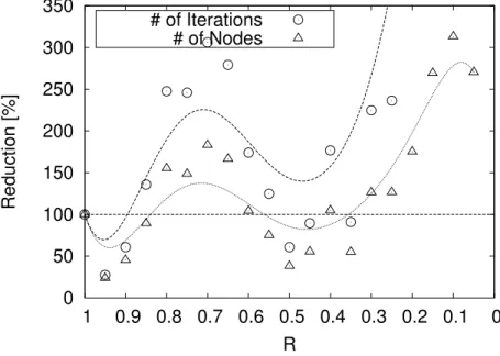
This is not the case forR = 0.0, because we cannot solve Hex(4) for this R when we limit ourselves to 500 million nodes. For ease of understanding, we prepare another graph in Fig 2-11. There we show the reduction rates normalized by the result of PN-search, i.e., the result of PN-search has 100% reduction rate.

Figure 2-11 shows that the number of iterations and nodes is reduced by a 30% reduction rate between R = 0.95 and R = 0.5. The result has two downward curves: from R = 1.0 to 0.7 and from R = 0.7 to R = 0.0. The first curve starts from R = 1.0 and decreases toward0.95. AfterR= 0.95, the results start to increase and grow to over 100%

after0.85. The second curve starts fromR = 0.7and the results starts to decrease again.

At aroundR = 0.5, the results reach about 50%. Finally, the results are increasing again

(42)

0 5000000 10000000 15000000 20000000 25000000 30000000 35000000 40000000

0 0.1 0.2 0.3 0.4 0.5 0.6 0.7 0.8 0.9 1

0

10000000 20000000 30000000 40000000 50000000 60000000 70000000 80000000 90000000 100000000

# of Iterations # of Nodes

R

# of Iterations

# of Nodes

Figure 2-10: The variation in Hex: The changes of Reducing and Increasing Cases for # of Iterations and # of Nodes [19]

0 50 100 150 200 250 300 350

0 0.1 0.2 0.3 0.4 0.5 0.6 0.7 0.8 0.9 1

Reduction [%]

R

# of Iterations

# of Nodes

Figure 2-11: The reduction rate in Hex: # of Iterations and # of Nodes for Hex(4).

toward R= 0.0, like Othello.

For understanding the details of how DeepPN works around R = 0.95, we tried to change R by 0.1 between from 1.0 to 0.9. The results are shown in Fig 2-12.

By looking at the results, we can see that DeepPN works almost twice as good as PN-search from R = 0.99 to 0.95. Form R = 0.95 to 0.90, we have a small curve like

(43)

0 20 40 60 80 100 120

0.9 0.91 0.92 0.93 0.94 0.95 0.96 0.97 0.98 0.99 1

Reduction [%]

R

# of Iterations

# of Nodes

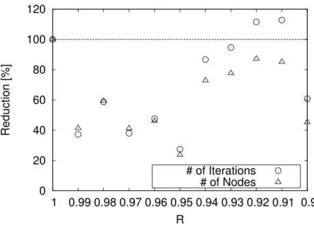
Figure 2-12: Hex: The detail of Fig 2-11. This figure is zoomed1.0≤R≤0.9. The lower is better. [19]

figure 2-11.

In Hex(4), the optimum value of R is around R = 0.95 (and perhaps R = 0.5). We can see that depth-first does not work so well for Hex(4) as it does for Othello, although there is an improvement over pure best-first.

Discussion

DeepPN works efficiently in 16-ply Othello endgame positions, and in Hex(4). It can reduce the number of iterations and nodes almost by half compared to PN-search. It must be noted that the optimum balance ofR is different in each game and for each size of game tree. We can see that for both games a certain amount of depth-first behavior is beneficial, but the changes are not the same. The precise relation is a topic of future work.

Both in Othello endgame positions and in Hex(4), we encountered positions that showed increasing (worse) results. We suspect that a reason for this problem may be (1) the holding problem and (2) the length of the shortest correct path. Concerning (1), the depth-first search can remain stuck in one subtree (holding on to the subtree). If this holding subtree cannot find the game-theoretical value, then the number of iterations and nodes become meaningless. When DeepPN employed a strong depth-first manner, then