JAIST Repository
https://dspace.jaist.ac.jp/
Title
確率的シソーラスと文書クラスタに基づいたトリガー
言語モデルの拡張による音声認識
Author(s)
Troncoso Alarcon, Carlos
CitationIssue Date
2003‑03
Type
Thesis or Dissertation
Text versionauthor
URL
http://hdl.handle.net/10119/1653
RightsDescription
Supervisor:下平 博, 情報科学研究科, 修士
An Extension to the Trigger Language Model Based on a Probabilistic Thesaurus and Document Clusters
for Automatic Speech Recognition
By Carlos Troncoso Alarc´ on
A thesis submitted to School of Information Science,
Japan Advanced Institute of Science and Technology, in partial fulfillment of the requirements
for the degree of
Master of Information Science
Graduate Program in Information Science
Written under the direction of Associate Professor Hiroshi Shimodaira
March, 2003
An Extension to the Trigger Language Model Based on a Probabilistic Thesaurus and Document Clusters
for Automatic Speech Recognition
By Carlos Troncoso Alarc´ on (110089)
A thesis submitted to School of Information Science,
Japan Advanced Institute of Science and Technology, in partial fulfillment of the requirements
for the degree of
Master of Information Science
Graduate Program in Information Science
Written under the direction of Associate Professor Hiroshi Shimodaira
and approved by
Associate Professor Hiroshi Shimodaira Professor Masato Akagi
Associate Professor Kentaro Torisawa
February, 2003 (Submitted)
Copyright c2003 by Carlos Troncoso Alarc´on
Abstract
In this work, an extension to the trigger-based language model (LM) for large vocabulary continuous speech recognition (LVCSR) is proposed. In this approach, instead of trigger pairs based on the average mutual information measure, related words extracted from a probabilistic thesaurus and document clusters, both created from a text corpus by us- ing EM-based clustering, are used. The probabilistic thesaurus captures syntactic and semantic relations between words, while the document clusters can provide information about the topic of discourse. Short-range dependencies from the baseline bigram + tri- gram model and long-range dependencies from the extended trigger model are integrated by interpolating the models, and the resulting LM score is used to rescore N-best lists. A little improvement in speech recognition accuracy over both the baseline and the model with only a cache component was obtained for a Japanese newspaper task.
Contents
Acknowledgments 1
1 Introduction 2
1.1 Background . . . 2
1.2 Motivation . . . 2
1.3 Thesis Organization . . . 3
2 Language Modeling 4 2.1 Introduction . . . 4
2.2 Language Models in Automatic Speech Recognition . . . 5
2.3 n-grams . . . . 6
2.4 Alternatives ton-grams . . . 7
2.4.1 Short Distance . . . 7
2.4.2 Intermediate Distance . . . 8
2.4.3 Long Distance . . . 8
2.5 Language Models Relevant to this Research . . . 9
2.5.1 The Cache-Based Language Model . . . 9
2.5.2 The Trigger Language Model . . . 10
2.6 N-best Rescoring . . . 11
2.7 Summary . . . 12
3 Extension Based on a Probabilistic Thesaurus 13 3.1 Probabilistic Thesaurus . . . 13
3.2 Methodology . . . 16
3.3 Experimental Environment . . . 17
3.4 Experimental Results . . . 17
3.4.1 Final Model . . . 18
3.4.2 Stop List . . . 18
3.4.3 Independent Components . . . 21
3.4.4 Words in 1-best Sentence . . . 23
3.5 Summary . . . 24
4 Further Extension Based on Document Clusters 25
4.1 Document Clusters . . . 25
4.2 Methodology . . . 26
4.3 Experimental Environment . . . 27
4.4 Experimental Results . . . 27
4.4.1 Final Model . . . 27
4.4.2 Cache Size . . . 29
4.4.3 Extension Based Solely on Document Clusters . . . 32
4.4.4 Assessing the Usefulness of the Related Words . . . 33
4.5 Results Analysis . . . 33
4.6 Summary . . . 36
5 Conclusions and Future Works 37 5.1 Conclusions . . . 37
5.2 Future Works . . . 38
Appendices 38
A Example of Classes in Probabilistic Thesaurus and Document Clusters 39
B Evaluation Data 41
List of Figures
2.1 The automatic speech recognition paradigm . . . 5
2.2 Cache-based language model . . . 10
2.3 Trigger language model . . . 11
3.1 Construction of the probabilistic thesaurus . . . 13
3.2 Outline of the extension based on a probabilistic thesaurus . . . 15
3.3 Speech recognition accuracy of the extension based on a probabilistic the- saurus, for different values of λ and a base cache size equal to 25 . . . 19
3.4 Speech recognition accuracy of the model with the stop list vs. the model without the stop list, for different values of λ and a base cache size equal to 25 . . . 20
3.5 Speech recognition accuracy of the model with a buffer, for different values of λ, a base cache size equal to 500 and a buffer size equal to 1250 . . . . . 22
3.6 Speech recognition accuracy of the model that uses the 1-best vs. the model that uses the 20-best, for different values of λ and a base cache size equal to 25 . . . 23
4.1 Outline of the further extension based on document clusters . . . 26
4.2 Speech recognition accuracy of the further extension based on document clusters, for different values of λ and a base cache size equal to 25 . . . 28
4.3 Maximum speech recognition accuracy of the two proposed extensions, for different values of the cache size . . . 30
4.4 Speech recognition accuracy forλ equal to 0.2 of the two proposed exten- sions, for different values of the cache size . . . 31
4.5 Speech recognition accuracy of the extension based solely on document clusters, for different values of λ and a base cache size equal to 25 . . . 32
4.6 Speech recognition accuracy of the further extension based on document clusters with erroneous classes, for different values of λ and a base cache size equal to 25 . . . 34
List of Tables
3.1 Experimental environment for the extension based on the probabilistic the- saurus . . . 18 4.1 Experimental environment for the further extension based on the document
clusters . . . 29 A.1 Examples of classes from the probabilistic thesaurus . . . 40 A.2 Examples of clusters from the document clusters . . . 40
Acknowledgments
The present research would have been impossible to complete without the help of many people.
First of all, I would like to thank the Japanese Ministry of Education, Culture, Sports, Science and Technology for giving me the opportunity to study in Japan.
I would also like to give many thanks to Professor Hiroshi Shimodaira and Mitsuru Nakai for their constant guidance, advice and support, and Professor Shigeki Sagayama for encouraging and accepting me for coming to Japan.
I am also very grateful to Professor Kentaro Torisawa, for his helpful ideas, support and for constructing the data on which my research is based, and to Shigeki Matsuda, for his bright ideas, C libraries and constant support.
Thanks go also to Professor Masato Akagi for supporting my research.
Many thanks to Hiroki Morimoto and Youichi Dohi, for recording the evaluation data for my research, and to Hiroo Nishiyama, for supervising the recording.
I’d also like to thank Dr. Masafumi Nishimura and his colleagues at IBM Tokyo Re- search Laboratory, for their feedback and help.
I owe a considerable debt of gratitude to my wife, Remedios Garc´ıa Bonilla, for her encouragement, understanding, and patience during my research.
I am particularly thankful to God, who has helped me in every moment.
Last, but not least, I would also like to take this opportunity to thank all my fellows in the laboratory and many other people at JAIST for their sincere help and cooperation.
Chapter 1 Introduction
1.1 Background
Automatic Speech Recognition (ASR) is typically based on two stochastic models: the acoustic model and the language model (LM). LMs are an important part of ASR systems, because they model the linguistic relations among words in the utterance that is to be recognized.
The most widely used LM in ASR is the n-gram model, where n typically equals 2 (bigram model) or 3 (trigram model). n-grams model the occurrence probability of n consecutive words in the text, and their parameters are estimated from a large text corpus.
n-gram models are very powerful in modeling dependencies between words that are adjacent or very near to each other within the text. However, they fail in modeling long-range dependencies between words, because they rely on a past word history limited to n −1 words. Nevertheless, it has proved very difficult to outperform these models, mainly due to their simplicity, and many attempts to model longer-range dependencies have resulted in a very little improvement in recognition accuracy.
One of the approaches that tried to cope with this limitation ofn-grams is the trigger LM [32]. This model uses a cache component similar to that of the cache-based LM [25], in which the most recent “rare” words are stored. In addition, a set of semantically related pairs of words called trigger pairs, constructed from a large text corpus by using the average mutual information measure, is also used. For every word in the cache, the model will predict a heightened probability not only for it, but also for all the words related to it through a trigger pair.
1.2 Motivation
The drawback of the trigger LM is that its performance is similar to that of the basic cache-based LM, because most of the best triggers are the so-calledself-triggersor triggers with the same root.
It seems reasonable to think that if the correlations between words were improved, we could have trigger pairs with a more significant effect in the overall system performance.
In this work, an extension of the trigger LM is proposed, in which, instead of trigger pairs, a probabilistic thesaurus of related pairs of words is used to extract words related to the one being processed. In addition, a further extension is proposed, in which related words from document clusters are also extracted and incorporated into the cache.
The probabilistic thesaurus incorporates to the model syntactic and semantic dependen- cies between words, while the document clusters can provide information about the topic of discourse. By taking advantage of the different features of these knowledge sources, this approach aims to improve the concept of trigger pairs with stronger word correlations, in order to improve the overall recognition accuracy in a typical speech recognition system.
1.3 Thesis Organization
This thesis is organized as follows. First, chapter 2 presents an introduction to statistical LMs, including those models relevant to this work, as well as the N-best rescoring par- adigm. Chapter 3 describes the proposed extension based on a probabilistic thesaurus, and shows the experimental results obtained for it. Chapter 4 proposes a further exten- sion based on document clusters, with its experimental results. Finally, in chapter 5 the conclusions and directions for future works are presented.
Chapter 2
Language Modeling
2.1 Introduction
Language modeling is the attempt to characterize, capture and exploit regularities in natural language [32]. Natural language is extremely difficult to model formally, due to its inherent variability and uncertainty.
There are two main approaches to language modeling: statistical language modeling and knowledge-based language modeling. The statistical approach tries to capture regularities in language from large amounts of text in a process known astraining. On the other hand, knowledge-based modeling uses a set of linguistic rules coded by experts, as well as domain knowledge, to assess the grammaticality of sentences.
The advantages of statistical language modeling over the knowledge-based approach are:
• Statistical models assign a probability to each possible sentence, while knowledge- based models usually only provide a “yes”/“no” answer to the grammaticality of a sentence. Probabilities convey much more information than such a simple answer.
Moreover, spoken language is often ungrammatical.
• Statistical models can be unexpensively built from a great variety of domains, as soon as the training procedure has been implemented.
• Coding linguistic rules by hand can be tedious and sometimes erroneous.
• At runtime, knowledge-based models like parsers are more computationally expen- sive than statistical models.
Statistical language modeling has also some disadvantages:
• They do not capture the meaning of the text. Therefore, they may assign a high probability to nonsensical sentences.
• Statistical models require large amounts of training data, which are not always available.
• Statistical language modeling often do not make use of linguistic and domain knowl- edge, which sometimes can be very helpful.
Language modeling is useful in areas like Automatic Speech Recognition (ASR), ma- chine translation and any other application that process natural language with incomplete knowledge. In this work, statistical language modeling is used for ASR.
2.2 Language Models in Automatic Speech Recogni- tion
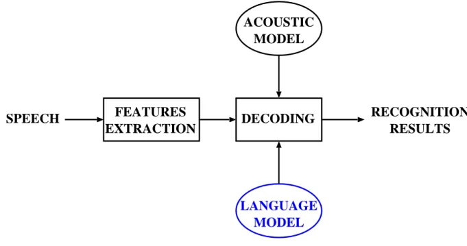
ASR is typically performed as follows. First, the features of the input speech signal are extracted via a spectral analysis. Then, based on the acoustic and the LM probabilities, the search for the best hypothesis is performed. The result of this search is the output of the ASR system. This paradigm is illustrated in figure 2.1.
ACOUSTIC MODEL
LANGUAGE MODEL FEATURES
EXTRACTION DECODING RECOGNITION RESULTS SPEECH
Figure 2.1: The automatic speech recognition paradigm
Probabilistically, the aim is to find the word sequenceW that maximizes the probability of a word sequence given the acoustic signal A. Applying the Bayes rule,
arg max
W P(W|A) = arg max
W
P(A|W)P(W)
P(A) = arg max
W P(A|W)P(W) (2.1) The calculation ofP(A|W) is the role of the acoustic model, whereas the LM is respon- sible for the computation of P(W).
Let W = w1n w1, w2, ..., wn, where the wi’s are the words that make up the word sequence. P(W) can be decomposed, by using the chain rule, in the following way:
P(W) =P(w1)
n
i=2
P(wi|w1i−1) (2.2)
Most statistical LMs try to estimate expressions of the form P(wi|h), where h wi1−1 is known as the history.
Since the number of possible histories that can precede a given word is very large, it is unfeasible to try to estimate the probability of all of them from the limited corpora that are available. Therefore, some simplification must be applied to the above equation.
Usually, the event space is partitioned in equivalence classes depending on some property of the text. For instance, in the trigram model the partition is based on the last two words of the history.
2.3 n-grams
An n-gram [1] is a model that uses the last n−1 words of the history as its sole infor- mation source. Typically nequals 2 or 3, and they are called bigram andtrigrammodels, respectively.
As commented in the previous section, n-gram models partition the data into equiv- alence classes based on the last n − 1 words of the history. Therefore, the following simplification is made:
P(wi|w1i−1) =P(wi|wii−1−n+1) (2.3) In this way, a bigram estimatesP(wi|h) by P(wi|wi−1), a trigram byP(wi|wi−2, wi−1), and so on.
n-grams are affected by the classic modeling tradeoff between detail and reliability.
When n is small, the parameters are reliably estimated from the training data, because the tuples are found easily. However, the modeling power is smaller than for greater values ofn. On the other hand, whenn is big, the data are insufficient and the estimates become unreliable. Nevertheless, the modeling power is bigger in this case.
The choice of n should depend on the amount of data available. For the sizes of the corpora typically available nowadays, trigrams own the best balance between reliability and detail, although interest is gradually moving towards 4-grams and beyond.
These models are easy to implement and easy to interface to the ASR decoder. They are very powerful and difficult to improve, mainly because of their simplicity. They seem to capture well short-range dependencies. It is for these reasons that they have become the standard LMs in ASR.
Unfortunately, they also have their drawbacks. First, they are unaware of any phenom- enon or constraint that is outside their limited scope. Therefore, they may assign high probabilities to nonsensical and even ungrammatical utterances, as long as they satisfy local constraints. In addition, the predictors inn-gram models are defined by their order
in the sentence, not by their linguistic properties. Therefore, histories like “the fireman extinguished the” and “the fireman extinguished quickly the” are very different for a trigram, even though they are very likely to precede the same word.
2.4 Alternatives to n-grams
There are many works in the literature that tried to overcome the mentioned limitations of n-grams. Below is a description of the most interesting approaches classified by the length of the scope they cover.
2.4.1 Short Distance
Class-based n-grams [3] aren-grams whose parameter space has been reduced by clus- tering the words into classes. The n-grams are then based on these classes, rather than the words themselves.
If it is assumed that each wordw belongs to only one class g(w), then this model can take many forms, for example,
P(wi|h) = P(wi|g(wi−2), g(wi−1)) (2.4) P(wi|h) = P(wi|g(wi−2), wi−1) (2.5) P(wi|h) = P(g(wi)|g(wi−2), g(wi−1))P(wi|g(wi)) (2.6) In practice, it is the last one that is the most used in class-based n-grams.
The clustering method itself can also take many forms.
Firstly, the clustering can be based on the linguistic knowledge. The best known ex- ample of this method is clustering by part of speech (POS). POS clustering attempts to capture syntactic dependencies between adjacent words in the text. This approach has several problems, though: some words can belong to more than one POS, POS classifica- tions made by linguists may not be optimal for language modeling, and there are many different schemes for POS classification.
In second place, in clustering by domain knowledge, all words that will behave in a similar fashion are manually grouped together. For example, days of the week, numbers, etc. This approach can be specially helpful when the amount of training data is limited.
Finally, in data-driven clustering, a large amount of data is used to automatically derive classes by statistical means. This is often better than clustering by hand based on one’s intuition. However, reliance on data instead of on external knowledge sources can also be problematic. For example, if the amount of training data available is not large enough, the resulting classes may not be reliable. The ideal data-driven clustering would be one supervised by an expert.
Class-basedn-grams have advantages over the basicn-grams. Since the possible number of histories is reduced, the model becomes more compact. Therefore, it could be expanded to include more context. For example, a class-based 4-gram model might be approximately
the same size as a trigram. In addition, since the number of classes is generally smaller than the size of the vocabulary, the data sparsity is reduced, and even if a word n-gram is not found in the training data, the equivalent class-based n-gram is likely to have been seen. For this reason, these models have been very helpful in situations where the training data available were limited.
The disadvantage of these models is that they lose some of the semantic information that word n-grams, however, capture. This can be partially overcome by constructing LMs that incorporate information from both word and class-based n-grams. A more important drawback of class-based n-grams is that they don’t solve the locality problem of n-grams.
2.4.2 Intermediate Distance
Long-distancen-grams[14] attempt to capture the dependencies between the predicted word andn−1-grams that are some distance back in the history. For instance, a distance- 2 trigram predicts wi based on (wi−3, wi−2). Distance-1 n-grams are consequently the conventional n-grams themselves.
These models have very serious limitations. Even though they capture dependencies between words that are separated by distance d, they cannot use different values of d at the same time during training, therefore, they unnecessarily fragment the training data.
In other words, they do not pay attention to the nature of the text in order to decide an appropriate value ford, but they simply skip the words that are nearer than dwords back in the history.
2.4.3 Long Distance
Mixture-based language models [5, 15] are composed of several LMs, each of which is specific to a particular topic or sublanguage. The probability distributions from these component LMs are linearly interpolated to form the global LM probability. The interpo- lation weights reflect, at each moment, which component sublanguage is currently being recognized.
LetM1, M2, ..., Mk be the component LMs. The overall LM probability is then P(wi|wi1−1) =
k
j=1
λjPMj(wi|wi1−1) (2.7) where the λj’s are the interpolation weights, with values such that
k
j=1
λj = 1 (2.8)
Usually, the first step when creating a mixture-based LM is the clustering: the training data has to be partitioned in homogeneous components. This can be done automatically,
with some iterative clustering algorithm, or manually, according to the topic, style of text, etc.
The number of clusters in which the training data should be partitioned is a delicate matter. A number too small will result in a model incapable of discerning between topics or linguistic styles in detail. Too large a number will lead to a bunch of undertrained models with poor probability estimates. It is common that one of the components be the whole training data, in order to smooth the estimates and avoid data fragmentation.
The next step is typically to construct an n-gram model for each of the constituents.
Then, the interpolation weights can be calculated by using the expectation maximization (EM) algorithm [10] in such a way as to maximize the likelihood of some held-out data.
These LMs are theoretically very attractive and represent a sound approach to LM adaptation. However, they have not significantly improved speech recognition accuracy so far.
Inside this category are also thecache-based language modeland the trigger lan- guage model, which are presented in the next section.
2.5 Language Models Relevant to this Research
From the various alternatives to n-grams presented above, the present research is partic- ularly based on the trigger LM, which in turn is based on the cache-based LM.
Both models are presented in this section.
2.5.1 The Cache-Based Language Model
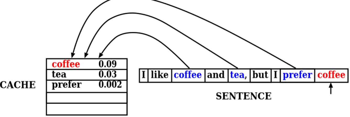
The cache-based LM [25, 26] is based on the observation that a word that has appeared recently in a document has a high probability of reappearing.
A cache memory similar to that of computers is used to store the words of recent appearance. The word probabilities are estimated from their recent frequency of use. If a candidate word is in the cache, its probability is raised.
Typically, a cache-based component is linearly interpolated with an n-gram LM:
P(wi|w1i−1) =λPcache(wi|w1i−1) + (1−λ)Pn−gram(wi|wi−n+ 1i−1) (2.9) Usually, a cache of the last K words is maintained, and the cache-based probability of a word is computed as the unigram probability of the word within the cache, that is,
Pcache(wi|w1i−1) = Ncache(wi)
K (2.10)
where Ncache(w) is the number of times w appears in the cache.
Figure 2.2 shows the outline of the cache-based model.
The original cache-based model was interpolated with a class-based trigram based on the POS, and a cache of size 200 was maintained for each POS. The interpolation weights were calculated individually for each POS.
coffee tea prefer
0.09 0.03 0.002
I like coffee and tea, but I prefer coffee CACHE
SENTENCE
Figure 2.2: Cache-based language model
Several extensions have been proposed to this LM, being the most obvious the addition of the cache-based component to a word-based trigram, rather than a class-based model [15].
The cache need not be limited to containing single words. Instead, recent bigrams and trigrams can also be incorporated to the cache and their probabilities boosted [18]. This approach has the problem that the probabilities ofn-grams in the cache cannot be reliably estimated due to the insufficient information contained in several hundred words back.
Another extension used the idea that the more recent words are more influential in predicting forthcoming words than those in the more distant past [5]. With this in mind, an exponentially decaying cache was constructed. This is a cache in which the probability of the words inside the cache decay exponentially with the distance from the word being predicted.
The cache-based LM significantly reduces the perplexity of standard LMs, and some of the extensions mentioned above contributed to a further improvement in terms of perplexity. However, the same does not apply to recognition accuracy, which has not been noticeably improved by this model so far.
2.5.2 The Trigger Language Model
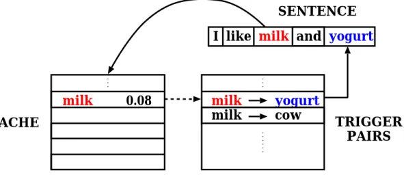
The trigger model [32, 33], like the cache-based model, also uses a cache memory of recent words. However, contrary to the original cache-based model, only “rare” words are incorporated to the cache. A word is defined as rare relative to a threshold of static unigram frequency.
In order to extract information from the document history, a basic information bearing element calledtrigger pairis used. If a wordais semantically well correlated with another word b, then (a →b) is called a trigger pair, with a being the trigger and b the triggered word. When a occurs in the cache, it triggers b, and the model will predict a heightened probability not only fora, but also for b.
The trigger pairs are created from a big text corpus by using the average mutual infor- mation measure:
I(a;b) = P(a, b) logP(b|a)
P(b) +P(a,¯b) logP(¯b|a) P(¯b) + P(¯a, b) logP(b|¯a)
P(b) +P(¯a,¯b) logP(¯b|¯a)
P(¯b) (2.11)
The model is formulated as a constraint of a maximum entropy (ME) framework [9, 16]
in which n-grams, long-distance n-grams and so on can also take part as constraints of the model.
The outline of this model is depicted in figure 2.3.
milk 0.08 CACHE
SENTENCE
milk yogurt milk cow
TRIGGER PAIRS I like milk and yogurt
Figure 2.3: Trigger language model
The drawback of trigger pairs is that far more information is contained in the self- triggers, that is, words that trigger themselves, than in any others; even the non-self- triggers tend to be triggers with the same stem (e.g. abuse, abused, abusing). Therefore, the improvement over the basic cache-based model is small.
2.6 N -best Rescoring
Most LMs that try to overcome the limitation of n-grams use a standard trigram or bigram-based speech recognizer to output the N-best list, that is, the N most likely hypotheses. Then, based on a combination of the scores provided by the speech recognizer and the new scores assigned by an alternative (generally more complex) LM, they perform a rescoring of the N-best list, reordering the hypotheses and proposing the most likely hypothesis as the output of the whole recognition process.
This process is called N-best rescoring, and it is widely used in language modeling for ASR, because of its easy implementation and fast evaluation.
In this work, N-best rescoring is also used.
2.7 Summary
An introduction to language modeling, with the two main approaches to language mod- eling and their pros and cons, has been presented in this chapter. The application of LMs to ASR, n-grams as the standard LMs and some alternatives to them have been discussed, with special emphasis given to the models relevant to this thesis. Finally, the N-best rescoring paradigm has been introduced.
In the next chapter, the proposed approach in detail is presented.
Chapter 3
Extension Based on a Probabilistic Thesaurus
3.1 Probabilistic Thesaurus
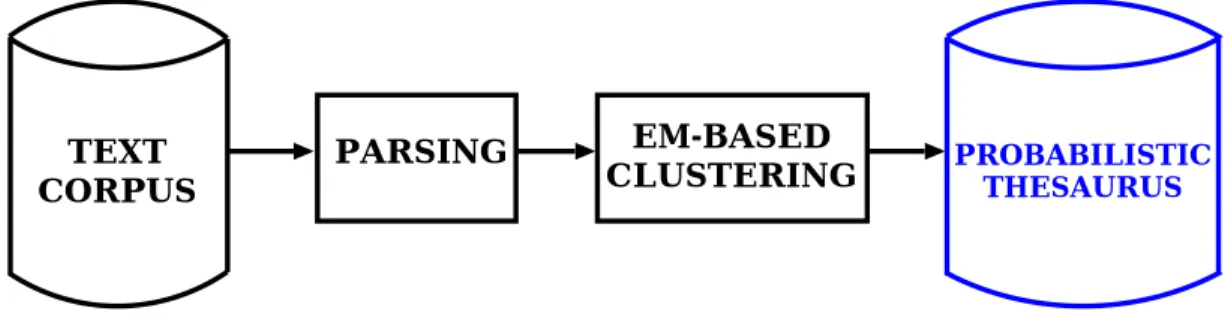
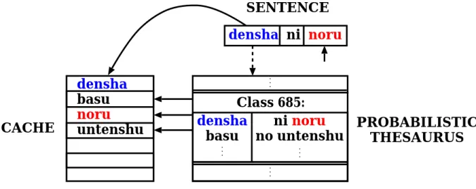
The probabilistic thesaurus [31, 43] consists of sets of words and related postposition + word pairs clustered in semantic classes, with their probability distributions (e.g. densha (train), basu (bus),... ↔ ni noru (to get on), no untenshu (driver),...). Each class is divided in two sets: a “leading words” set, i.e. words semantically related to each other, and a related words set, i.e. words related to the leading words set through a postposition (see Appendix A).
This thesaurus was automatically created from a large text corpus, namely, five and nine years of two Japanese newspapers, by using a statistical parser and EM algorithm-based clustering. Figure 3.1 illustrates this procedure.
TEXT CORPUS
PARSING EM-BASED
CLUSTERING PROBABILISTIC THESAURUS
Figure 3.1: Construction of the probabilistic thesaurus
This method used triples of the form < r, rel, l > as learning data, where r was a related word, l a leading word and rel the relationship between r and l. rel could be a postposition, a relative clause marker or an empty marker. The relative clause marker refers to the relation between the head verb of a given relative clause and its head noun.
The empty marker expresses the relation between words related to each other without the help of a postposition.
Each triple was divided in two items, < r, rel > and l. The probability that the triple occurred was defined as follows:
P(< r, rel, l >)
a∈A
P(< r, rel >|a)P(l|a)P(a) (3.1) where a denoted a class of the occurrences and A the set of all classes. The number of classes was fixed a-priori.
The EM-based clustering method estimates P(< r, rel >|a), P(l|a) andP(a) for each related wordr, leading wordl, relationshipreland classa. Unfortunately, this estimation is not straightforward, because the class a is not observed in the training data.
The following iterative algorithm was used to estimate the probabilities. First, a statis- tical parser was used to obtain a set of parse trees that capture the co-occurrence relations observed in the corpus. Then, the following list was created:
Q={< r0, rel0, l0>, < r1, rel1, l1 >, ..., < rn, reln, ln>} (3.2) The likelihood that Q is observed was calculated by the following formula:
<ri,reli,li>∈Q
P(< r, rel, l >) =
<ri,reli,li>∈Q
a∈A
P(< ri, reli >|a)P(li|a)P(a)
(3.3) The EM algorithm maximized the above probability by adjusting the parameters{P(<
r, rel > |a)|r ∈ R, rel ∈ Rel, a ∈ A} ∪ {P(l|a)|l ∈ L, a ∈ A} ∪ {P(a)|a ∈ A} iteratively, where R is the set of all related words, Rel the set of all relations and L the set of all leading words. The iteration continued until convergence or near-convergence of the likelihood.
The probabilities at the j-th iteration step were calculated as follows:
Pj(a|< r, rel >, l) = Pj(a)Pj(< r, rel >|a)Pj(l|a)
a∈APj(a)Pj(< r, rel >|a)Pj(l|a) (3.4) Based on the above formula, the probabilities at stepj+1 are computed in the following way:
Pj+1(a) = 1
|L|
<ri,reli,li>∈Q
Pj(a|< r, rel >, l) (3.5) Pj+1(< r, rel >|a) =
<r,rel,li>∈QPj(a|< r, rel >, li)
<ri,reli,li>∈QPj(a|< ri, reli >, li) (3.6) Pj+1(l|a) =
<ri,reli,l>∈QPj(a|< ri, reli >, l)
<ri,reli,li>∈QPj(a|< ri, reli >, li) (3.7) The probabilities of the last iteration are the output of the entire learning process.
The probabilistic thesaurus captures the syntactic and semantic relations between strongly correlated words better than trigger pairs.
In the proposed approach, for each word that is added to the cache, the most likely leading words and the most likely related words, without the postposition, from the most likely classes related to that word in the probabilistic thesaurus are also added to the cache. In this way, these words are incorporated into the cache component of the proposed model, so that they can help improve the predictors.
If a word is a verbalized noun +suru or an inflected form of a verb, only the base form is used. For example, frombenkyou suru(to study) onlybenkyou(study) is used, and from tsukawareru(to be used) only the base formtsukau(to use) is employed. By applying this generalization, the algorithm can compare the base form of the verbs in the cache with that of the verbs in the hypotheses during the N-best rescoring procedure, and thus, the prediction power of the verbs is raised. For example, in the sentences terebi wo miru (I watch TV) and terebi wo mita (I watched TV), it seems reasonable that the correlation between terebi (TV) and miru (to watch) should be used in both cases. Furthermore, when looking up in the probabilistic thesaurus, it is also desirable to use the base form of verbs, as we do when we look up a word in a dictionary.
Figure 3.2 shows the outline of the proposed model.
densha basu noru untenshu
densha ni noru
CACHE
SENTENCE
PROBABILISTIC THESAURUS Class 685:
densha basu
ni noru no untenshu
Figure 3.2: Outline of the extension based on a probabilistic thesaurus
The main differences between the trigger LM and the proposed approach are the fol- lowing.
First, the models use different data. The trigger pairs are pairs of well-correlated words that can be found in similar contexts (e.g. education→academic). On the other hand, the probabilistic thesaurus groups pairs of words syntactically related through a postposition in semantic classes. It reflects different uses of words (e.g. Daiei can be the name of a department store or the name of a baseball team).
In addition, the proposed model should model better the syntactic and semantic rela- tions between strongly correlated nouns and verbs (e.g. biiru(beer) ↔ nomu(to drink)),
pairs of nouns (e.g. Kyojin(Giants) ↔ toushu (pitcher)), etc.
3.2 Methodology
The proposed approach rescores the N-best hypotheses output by an ASR system using the scores provided by the new LM.
The rescoring algorithm proceeds as follows.
1. Read 1-best sentence
2. Add to the cache all words in the sentence
3. For each word in the sentence, add to the cache the most significant related words from the probabilistic thesaurus
4. For each hypothesis in the N-best:
• Calculate the score of the extended cache component
• Calculate the score of the proposed LM
• Calculate the total score (acoustic model + proposed LM) 5. Output the hypothesis with the highest total score
Here, by “significant” I mean “with the highest probability”.
The total score is the score of the acoustic model output by the speech recognizer times the score of the proposed LM.
The score of the proposed LM is the interpolation between the score of the extended cache component and the baseline LM score output by the speech recognizer, that is,
S(W) = Sextended(W)λSbaseline(W)1−λ (3.8)
where λ is the interpolation weight and W is the sentence being processed. In this way, one can take advantage of the short-range dependencies modeled by the baseline model and add the longer-range dependencies that the proposed model captures.
We define the score of the extended cache component as the normalized product of the cache score for all the words in the sentence. Since the length of the sentences within the N-best is variable, the score needs to be normalized. I propose the following way:
Sextended(W) =
n
i=1
(Scache(wi))mn (3.9)
where wi are the words that compose W, n is the length (number of words) ofW and m is the average length of the N-best sentences.
For every word, the cache score is defined as the unigram probability inside the cache if the word belongs to the cache, and a value close to 0, ε, otherwise, as follows:
Scache(wi) =
N
cache(wi)
Cache Size Ncache(wi)= 0
ε otherwise (3.10)
where Ncache(w) is the number of times w appears in the cache.
3.3 Experimental Environment
Experiments with two different test data sets of the same 71 sentences from two different male speakers were conducted. These test data consisted of an article about education from the Japanese Yomiuri Shimbun newspaper (see Appendix B). These data were not used to create the probabilistic thesaurus or the document clusters.
The ASR system Julius 3.1 [21] was used to output the N-best hypotheses that the model rescores, where N was set to 100. This system performs a two-pass (forward- backward) search using a back-off bigram and a back-off trigram model in the respective passes, with a cut-off threshold of 1 for both models. These models were trained from 75 months (01/1991-09/1994, 01/1995-06/1997) of the Japanese Mainichi Shimbun newspa- per. A vocabulary of 21322 words was used.
The recognition accuracy for this baseline model was 89.72% for test set 1 and 85.10%
for test set 2. The average recognition accuracy of the baseline model is thus 87.41%.
The maximum recognition accuracy that can be attained by choosing the best hypothe- sis from theN-best each time is 93.54% for test set 1 and 89.16% for test set 2. Therefore, the average maximum attainable accuracy is 91.35%.
The value ofε in equation 3.10 was set to 10−30.
Five years (1991-1995) of the Japanese Mainichi Shimbun newspaper and nine years (1990-1998) of the Japanese Nihon Keizai Shimbun newspaper were used to construct the probabilistic thesaurus.
The number of significant classes from the 2500 in the probabilistic thesaurus was 5, and the number of significant leading words and significant related words for each class were also 5 each. Therefore, for every word that is added to the cache, 50 related words are also added, and consequently, the cache size for the proposed model is 51 times the size of that for the model with only a cache component.
The previous parameters were empirically tuned.
The speech recognition accuracy for the model with only the cache component and the extended trigger model based on the probabilistic thesaurus was computed for values of λ from 0 to 1 incremented by 0.05, and base cache sizes equal to 5, 10, 25, 50, 100, 250 and 500.
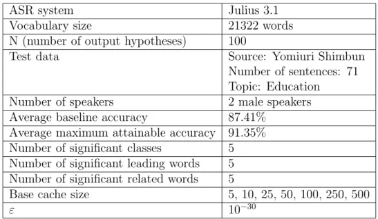
The experimental environment is summarized in table 3.1.
3.4 Experimental Results
Many experiments were carried out in this research. Some were used to tune the model parameters, like those described in the previous section, others used a-priori assumptions,
ASR system Julius 3.1
Vocabulary size 21322 words
N (number of output hypotheses) 100
Test data Source: Yomiuri Shimbun
Number of sentences: 71 Topic: Education
Number of speakers 2 male speakers
Average baseline accuracy 87.41%
Average maximum attainable accuracy 91.35%
Number of significant classes 5 Number of significant leading words 5 Number of significant related words 5
Base cache size 5, 10, 25, 50, 100, 250, 500
ε 10−30
Table 3.1: Experimental environment for the extension based on the probabilistic the- saurus
which turned out to be erroneous, and others tried different data or different methods of combining the model parameters.
In this section, the basis for these experiments and the results obtained are described.
3.4.1 Final Model
The proposed model was tested against a model that only uses the cache component, that is, it does not add to the cache any related words.
The maximum recognition accuracy of the proposed model was obtained for a cache size of 25 for both data sets, and the average of the results of the experiments from the two sets for this cache size is shown in figure 3.3.
It can be observed that, for certain values of λ, the extended trigger model based on the probabilistic thesaurus has a higher recognition accuracy than both the baseline and the model with the cache component alone. An improvement of 0.31% (absolute) over the baseline was obtained, which represents a 7.9% of the total possible improvement.
This improvement, although not very significative, may mean that the related words extracted from the probabilistic thesaurus constitute indeed a useful external source for the LM. In the next chapter, an experiment will try to confirm the usefulness of these related words.
3.4.2 Stop List
It is not hard to realize that function words, like Japanese postpositions or auxiliary verbs, are somewhat uniformly distributed all over a given text. On the other hand, the frequency of appearance of content words usually depends on linguistic properties of the
87 88 89 90 91
0 0.2 0.4 0.6 0.8 1
Recognition accuracy (%)
λ
Maximum attainable accuracy P.T.
Cache Baseline
Figure 3.3: Speech recognition accuracy of the extension based on a probabilistic the- saurus, for different values of λ and a base cache size equal to 25
text like the topic of discourse, the type of text, etc. Consider, for example, the word
“pitcher”. It is obvious that it will appear with a greater frequency in a sports article than in one about religion.
Initially in this research, the assumption that content words would have a greater impact in the cache than function words was made. Therefore, a stop list, that is, a list of function words that are not incorporated into the cache nor used to look for related words, was constructed.
The stop list was created from a large text corpus of Japanese newspapers by inserting in the list all the words with a frequency higher than or equal to 260. This threshold was fixed by hand to meet the requirement that no content words, except those that frequently appear in Japanese newspapers likenihon(Japan),keizai(economy) orbeikoku(America), appeared in the list. The list contains 92 words.
Experiments refuted this hypothesis, as shown in figure 3.4, where it can be seen that the model with an empty stop list performed much better than the one with the non-empty list.
87 88 89 90 91
0 0.2 0.4 0.6 0.8 1
Recognition accuracy (%)
λ
Maximum attainable accuracy P.T. without Stop List P.T. with Stop List Baseline
Figure 3.4: Speech recognition accuracy of the model with the stop list vs. the model without the stop list, for different values ofλ and a base cache size equal to 25
The possible reason for this counterexample can be that the absence of function words
in the cache makes the cache component assign a very low probability to function words in the hypothesis, therefore, sentences with fewer function words, like erroneous sentences with less function words than normal, are assigned higher probabilities, and consequently the recognition accuracy drops.
3.4.3 Independent Components
In the original trigger LM, the words triggered by those in the cache are not incorporated into the cache, as opposed to the proposed approach. In the original model, the trigger pairs are stored apart from the cache, and the words that are in the cache are looked up in them.
On the other hand, in the proposed model, the words that are added to the cache are looked up in the probabilistic thesaurus, and the related words are inserted in the cache.
Two different experiments were performed, in which analogously to the original trigger model, the related words were not incorporated into the cache.
In the first experiment, for all the words in the cache, a list of related words was generated and stored apart. Then, the cache score and the trigger score were computed separately and interpolated with the baseline score by means of the following formula:
S(W) =Scache(W)λ1Srelated(W)λ2Sbaseline(W)λ3 (3.11) The cache score was computed in the same way as in equation 3.10.
The score of related words was defined as follows:
Srelated(W) =
n
i=1
(Srelated(wi))mn (3.12)
where n is the length of W and m is the average length of theN-best sentences.
Srelated(wi) =
N
related(wi)
Cache Size Nrelated(wi)= 0
ε otherwise (3.13)
where Nrelated(w) is the number of times w appears in the related words list.
This model did not perform better than the final one for any of the cache sizes tried.
In the second experiment, the words with more recent appearance were stored both in the cache and in a word buffer smaller than the cache. Then, instead of creating the list of related words from the cache, it was created by looking up the words in the buffer in the thesaurus. In this way, the size of the cache is made independent of the number of words that take part in the thesaurus lookup.
The scores were computed as in the experiment above.
Analogously to the previous experiment, this approach did not help to improve the recognition accuracy.
There can be several reasons for the underperformance of these two approaches. One possible cause can be in the interpolation scheme: the interpolation weights might not be optimal, or the magnitude of the scores could be very different. Another possible problem
can be the score of the related words itself. It has been defined exactly in the same way as the cache score, but it might not be useful to use the unigram probability of the related words. The usage of the probability distributions of the words in the probabilistic thesaurus seems more reasonable. These matters will be dealt with in future works.
Using the same word buffer as that of the last mentioned approach, another experiment was tried, where the model components were no longer independent, but the only related words that were added to the cache were those triggered by the words in the buffer. Thus, in this approach the cache size is also independent of the number of words that are looked up, but all the words end up together inside the cache.
Different sizes for the cache and the word buffer were tried. The sizes that achieved the best results were 1250 for the buffer and 500 for the cache. Observe that 1250 is 25 times 50, that is, almost the same size as that of the cache of the final model. The results for these sizes are presented in figure 3.5.
87 88 89 90 91
0 0.2 0.4 0.6 0.8 1
Recognition accuracy (%)
λ
Maximum attainable accuracy P.T. without Word Buffer P.T. with Word Buffer Baseline
Figure 3.5: Speech recognition accuracy of the model with a buffer, for different values of λ, a base cache size equal to 500 and a buffer size equal to 1250
As it can be seen, this approach did not outperform the proposed model. As the parameters were made closer to those of the final model, the recognition accuracy was improved. This means that the final model behaves better than this approach.
3.4.4 Words in 1-best Sentence
As mentioned in section 3.2, the proposed model uses the words in the 1-best sentence for the cache component, and the related words from the probabilistic thesaurus are based on them too.
The 1-best sentence normally contains errors. If it didn’t, it would not be necessary to improve the LM. It may then seem unappropriate to use the words in that sentence for the cache component, because a misrecognized word in the cache may contribute to incur the same error again, since the probability of the erroneous word may be raised over that of the correct one.
With this in mind, a modification to the algorithm was made. In it, instead of using the words in the 1-best sentence, the words that appeared more than 10 times within the 20-best sentences were used. This figures were optimized empirically.
The results of this experiment are shown in figure 3.6.
87 88 89 90 91
0 0.2 0.4 0.6 0.8 1
Recognition accuracy (%)
λ
Maximum attainable accuracy P.T. with 1-best P.T. with 20-best Baseline
Figure 3.6: Speech recognition accuracy of the model that uses the 1-best vs. the model that uses the 20-best, for different values of λ and a base cache size equal to 25
It didn’t come as a surprise the fact that the described modification did not improve the results, because there are several works with similar results [7].
3.5 Summary
In this chapter, an extension to the trigger LM based on a probabilistic thesaurus has been presented. The features of the probabilistic thesaurus, the main differences with respect to the original trigger LM and the methodology of the proposed approach have been discussed. Finally, the experimental environment used in this research, as well as several different experiments, with their corresponding results, have been detailed.
In chapter 4, an additional extension to the approach that has been discussed here is presented.
Chapter 4
Further Extension Based on Document Clusters
4.1 Document Clusters
The document clusters [13] consist of clusters of documents with similar contents along with words that are likely to appear in these documents, with their probability distribu- tions (e.g. document 573, document 947,... ↔densha(train),eki(station), sen(line),...).
They were also created by means of EM-based clustering from a text corpus different to that used for the probabilistic thesaurus, in this case, five years of a different Japanese newspaper.
The algorithm used for creating these data was the same as in the probabilistic the- saurus, except that, in this case, the method used pairs of the form < d, w >, where d denoted a document and w a word.
Then, the probability was defined as P(< d, w >)
a∈A
P(d|a)P(w|a)P(a) (4.1) where a denoted a class of the occurrences andA the set of all classes.
The document clusters can specify the words that are likely to denote major topics in a set of similar documents.
Like in the approach presented in the previous chapter, for each word that is added to the cache, the most likely leading words and related words, without the postposition, from the most likely classes for that word in the probabilistic thesaurus are also added to the cache. In addition, the most likely words from the most likely clusters for that word in the document clusters are also incorporated into the cache if they are not already in it.
Figure 4.1 shows the outline of the proposed model.
The main differences between the probabilistic thesaurus and the document clusters are the following.
The probabilistic thesaurus captures syntactic and semantic relations between corre- lated pairs of words, while the document clusters capture topic constraints, such as word
densha basu noru untenshu eki
sen
densha no untenshu wa eki ni iru
CACHE
SENTENCE
PROBABILISTIC THESAURUS
Class 685:
densha basu
ni noru no untenshu Cluster 189:
densha eki sen
DOCUMENT CLUSTERS doc 573
doc 947
Figure 4.1: Outline of the further extension based on document clusters choice and co-occurrence patterns.
The leading words set in the probabilistic thesaurus is associated to the related words set through a postposition, and the words in the former set are very likely to be found in the text followed by the corresponding words in the latter set. However, the related words in the document clusters are not syntactically related to each other, so they simply constitute a set of semantically related words, which may well belong to the same topic of discourse.
Consider as an example, that of figure 4.1. densha (train) andbasu (bus) can be easily found in the text precedingni noru (to get on) orno untenshu (driver), like in densha no untenshu (the train driver) or basu ni noru (to get on the bus). However, eki (station), although strongly associated to denshaas well, is not usually followed by ni noru (to get on). Therefore, eki will probably not appear in class 685 of the probabilistic thesaurus.
Consequently, the two knowledge sources can be complementary to each other and provide different features to the LM.
4.2 Methodology
The rescoring algorithm proceeds as follows.
1. Read 1-best sentence
2. Add to the cache all words in the sentence
3. For each word in the sentence, add to the cache the most significant related words from the probabilistic thesaurus
4. For each word in the sentence, add to the cache the most significant related words from the document clusters, if they are not already in the cache
5. For each hypothesis in the N-best:
• Calculate the score of the extended cache component
• Calculate the score of the proposed LM
• Calculate the total score (acoustic model + proposed LM) 6. Output the hypothesis with the highest total score
The scores in this further extension are calculated exactly in the same way as in the previous chapter.
4.3 Experimental Environment
The environment of the experiments that were conducted to test this model is almost the same as that of the previous chapter. Only the new parameters are presented here.
The document clusters were created from five years (1996-2000) of the Japanese Yomiuri Shimbun newspaper.
The number of significant clusters from the 300 document clusters was 1, and the number of significant words for each cluster was 5. Therefore, for every word that is added to the cache, 55 related words are also added, and consequently, the cache size for the proposed model is 56 times the size of that for the standard cache-based model.
The speech recognition accuracy for the extended trigger model based on both the probabilistic thesaurus and the document clusters was computed for values of λ from 0 to 1 incremented by 0.05, and base cache sizes equal to 5, 10, 25, 50, 100, 250 and 500.
The experimental environment is summarized in table 4.1.
4.4 Experimental Results
4.4.1 Final Model
The proposed extension was tested against the approach in the previous chapter and the model with only the cache component.
The average results of the experiments from the two sets, for a base cache size equal to 25, are shown in figure 4.2.
As it was also shown in the previous chapter, it can be observed that the extended trigger model based on the probabilistic thesaurus has a higher accuracy than both the baseline and the model with only the cache component. Furthermore, the extended trigger model based on both the probabilistic thesaurus and the document clusters has even a higher accuracy than the one based only on the probabilistic thesaurus. An improvement
87 88 89 90 91
0 0.2 0.4 0.6 0.8 1
Recognition accuracy (%)
λ
Maximum attainable accuracy P.T. + D.C.
P.T.
Cache Baseline
Figure 4.2: Speech recognition accuracy of the further extension based on document clusters, for different values of λ and a base cache size equal to 25
ASR system Julius 3.1
Vocabulary size 21322 words
N (number of output hypotheses) 100
Test data Source: Yomiuri Shimbun
Number of sentences: 71 Topic: Education
Number of speakers 2 male speakers
Average baseline accuracy 87.41%
Average maximum attainable accuracy 91.35%
Number of significant classes (P.T.) 5 Number of significant leading words (P.T.) 5 Number of significant related words (P.T.) 5 Number of significant clusters (D.C.) 1 Number of significant related words (D.C.) 5
Base cache size 5, 10, 25, 50, 100, 250, 500
ε 10−30
Table 4.1: Experimental environment for the further extension based on the document clusters
of 0.53% (absolute) over the baseline was obtained, which represents a 13.5% of the total possible improvement.
This additional improvement over the approach proposed in the previous chapter seems to prove that the additional related words extracted from the document clusters also contribute to improve the predictors in the LM. In the experimental results section this will be discussed again.
4.4.2 Cache Size
As it was previously commented, experiments with different cache sizes were performed.
Specifically, sizes of 5, 10, 25, 50, 100, 250 and 500 were tried. Remember that these sizes are later multiplied by the number of related words that are incorporated into the cache for each word that enters the cache (51 in the probabilistic thesaurus case and 56 if it is the model based on both the thesaurus and the document clusters).
Figure 4.3 shows the maximum recognition accuracy of the extension based on the probabilistic thesaurus and of the further extension based on the document clusters, for the different sizes of the cache. In figure 4.4 the speech recognition accuracy of both models for a fixed λ equal to 0.2 for the different cache sizes is illustrated.
In both cases, the higher recognition accuracy was achieved for a base cache of size equal to 25. This is why the cache size in the final models were set to this value.
87 87.2 87.4 87.6 87.8 88 88.2 88.4
5 10 25 50 100 250 500
Recognition accuracy (%)
Cache size
P.T. + D.C.
P.T.
Figure 4.3: Maximum speech recognition accuracy of the two proposed extensions, for different values of the cache size
87 87.2 87.4 87.6 87.8 88 88.2 88.4
5 10 25 50 100 250 500
Recognition accuracy (%)
Cache size
P.T. + D.C.
P.T.
Figure 4.4: Speech recognition accuracy forλequal to 0.2 of the two proposed extensions, for different values of the cache size
4.4.3 Extension Based Solely on Document Clusters
For the purpose of comparison, a model based solely on the document clusters was con- structed. The model is analogous to the one based only on the probabilistic thesaurus, that is, the related words that are incorporated into the cache are only the ones found in the document clusters.
This time, the number of significant clusters was set to 1, and the number of related words extracted from each cluster was 20. Therefore, for each word that enters the cache, 20 related words are also added, and thus the base size of the cache is multiplied by 21.
The average results are illustrated in figure 4.5.
87 88 89 90 91
0 0.2 0.4 0.6 0.8 1
Recognition accuracy (%)
λ
Maximum attainable accuracy P.T. + D.C.
P.T.
D.C.
Cache Baseline
Figure 4.5: Speech recognition accuracy of the extension based solely on document clus- ters, for different values of λ and a base cache size equal to 25
As it can be seen, the model based on the document clusters alone performs also slightly better than the model with only the cache-based component, but worse than the model based on the probabilistic thesaurus and the one based on the two knowledge sources.
This may mean that the document clusters have a less significative effect in the model than the probabilistic thesaurus.
In the next section, the usefulness of each of the model components is analyzed in more detail.