Simulated Annealing Programming Using Effective Subtrees

(1)

Simulated Annealing Programming Using Effective Subtrees

Yuichiro UÊDA^* , Mitsunori MÎKI^** and Tomoyuki HÎROYASU^***

(Received October 20, 2008)

Simulated Annealing Programming (SAP), an automatic programming method, is an extension method of Simulated Annealing (SA) that allows SA to handle tree structures. In this method, the point to exchange is chosen randomly, and the subtree to insert is also generated randomly. In this paper, we propose the method that finds out effective subtrees in search and that uses them to generate subtree for inserting. The proposal method can perform search more efficiently than standard SAP in Santa Fe trail problem and Symbolic Regression problem.

Key words automatic programming, program search, genetic programming, simulated annealing, effective subtrees

!"$#%'&()*#,+

-./01

243457698 :7;9<9= >7?9@ ACB

D E7FHGJI9K L MON9P9I Q7R9SUT4V9S9W E7R9S

XHY[Z]\_^_`ba_c_d]e_`bf_g_h]i

1. ^jklm

no&oprqstuvwxyz{t}|~

t |wx }q

,$

x

z ¡¢£¤

x¥¦§qno&

p

¨©

ªwx«¬z}¦zt¯®°

¡|wxy±

x²o

x}q«¬³z $

³q´µ,±¶r}o

·

Genetic Programming: GP^¸ ¹⁾¥ ³!o"$#%'&o(

* Graduate Student, Department of Knowledge Engineering and Computer Sciences, Doshisha University, Kyoto Telephone:+81-774-65-6921, Fax:+81-774-65-6716, E-mail:[email protected]

** Department of Knowledge Engineering and Computer Sciences, Doshisha University, Kyoto Telephone:+81-774-65-6930, Fax:+81-774-65-6716, E-mail:[email protected]

*** Faculty of Life and Medical Sciences, Doshisha University, Kyoto

Telephone:+81-774-65-6932, Fax:+81-774-65-6019, E-mail:[email protected]

)¹*¯#º+¯¯¯¯¯¹¯

·

Simulated Annealing Programming: SAP^¸ ²⁾ ^»¼½ ^x

GP^¿¾yÀ ^{z ry³¿´yµ} ^xy GP

q¹¯

§¯ÁÂ

¯ÃÄ

ADF³⁾^¥¯ÅÇÆ

/0¯1È

É

´¯µ 4)Ê¹#Ë(q¹Ì¯Å¯Í¡¹Î¯Ï½ÂÑÐÒ 5) ^zÇ{¡

«yÓ³q .ÔÕ

tÖ×,¶$xØ¶¶

GP

}

ÙÚ

¡Û

yqÜÝÞ

³ß

¡

àá

wxãâåä#pçæ

è

xä#p

qé

ê

¥Ösëìq àá

¡Ûz

Ä GP^qí

á

qîïð

±

x 6)

(2)

SAP ^ä# ^pq ^è ^xÐÒÇt

z´µ

Ä ,¡«yÓ³

»¼,$

² SAP

äy#p

è

³x±³zÂ

GP ^±q

x 2)^{¶¶ q} SAP^¡Ãxq ^è

µ¡ ¶$

$

Ã, ¡

è

¶$² /01

ty y¡ ,¶$²yÐ !ðo¡" #wox

µ

±

xq²o

.Ô

¡ Ù%$

z&

x

'

(

¡

-.

z

/01 ·) *

-

.¯/¯0¯1

±,+.-

¸

t¯0/¯¡

É

Û0¯Æ¹w

µÇt2103¹

t è wx

/y01

¡³£,¶r 4ywxy±

SAP

qq .ÔÕ

t5x

2. ⁶⁷⁸⁹

:%;½=<>@?ABC DBE

7

AB

F

SAP^G SAP

SA^t

1 H I J

3x«¬¡K L,¶$²´µ

x

)M

¡ SAPq)NO+ÞtPwØ

STEP 1 ^QRS ^q

è

QRS

t¡

è

¶

'

qTUts½¬

STEP 2

è VW

× Xoq

S

¡³£,¶$

GPqY Z [ \,±]q^ªt³s

¬±

_

¶$

S ` a t è

¶$

'

tT Uwxcb

d

o¡

Fig. 1¡P'¶$²o«o¬³¡³× Xoq

S

¡³£,¶ro

¡Y Z [ \ð

·

Ð !ð

¸

t ,¶$

'

qðte

±$wx /01

tf gwx

'

qhØ ¡ /01

t è

¶f g½¶² /0

¡"#wx

mutation point ųᲢrandomlyᲣ

select delete a subtree insert new subtree generate randomly

Fig. 1. Generation Method in SAP.

STEP 3 ⁱ

Wj

kl

× Xq

S

qT U m

E ^±

_

¶$

S ` a

qT U m

E⁰ ^±

q2n

0

∆E(=E⁰−E)^{ÃÇ«2o.p¯Í} T ^t¹ÎÇ¡

_ ¶

S ` a t i W

wxq

j ·i

W j ¸

ts,¬ i

W j ¡

q

(1)^¡Pw Metropolis^{Î r} ⁷⁾ ^tx

PAC=

1 if∆E≤0

exp(−^∆E_T ) otherwise (1)

STEP 4 ^s ^#½+

STEP2 ^Ão«to 3^t

R

ìu Äwv'¶ ² hytpyÍ

T

tx

Â$wx

s

#,+hqpÍ

Tk+1

q ·

2^¸

¡«Óy

wx

Tk+1=γTk (0.8≤γ <1) (2)

γ

z{

Ô

Ä

Tk

× XqpÍ

x

STEP 5 ^|}

j

STEP2^~ 4^t ^²§s3t ^|} ^wx

3.

(

GP^q

¾À

z #

s

îï

x Santa Fe trail^îï ¹⁾^Ã«o Symbolic Regression

îï 1) ^{t£ ½±¶$²} Santa Fe trail^îï

H

Ý

,p$

È è

wxîïwoz

S

tT Uwx

¡Ös

$

z³Ê#(

%$³

x& qyxîï

x Symbolic Regression^îï

H

Ýºp¯

È è

¶zîïwz w qÊ#(

S q

TU¡twîï

x

3.1 Santa Fe trail

Santa Fe trail^îï½± 1 ^q. Fig. 2(a)

¡Pw 32 32 ^q

t

¡

¿

² t

² %¡ N£¢y#£¤

o'

x ¥£Á Â¦

w,xo

ooot è

w'xoîï

ox 1)^zyÃow

q ,t ¦ w

o

%§

¶² ±w'x¨

| ©

ª¬«

{IF FOOD AHEAD, PROGN2, PROGN3}

|©

ª®«

{LEFT, RIGHT, MOVE} ^x IF FOOD AHEAD

¯

§ot 2Û °%³} oq

1

±

¡

² 1^¯ ^§tz ^² 2^¯ ^§t

Ö¯s¯wx¯

PROGNn^.¯ ^§Çt n^³ ^°0¹.² 1 ^¯ ^§¯

² 2

¯

§¯ · · ·^² n

¯

§Çq´¡¹Öswx¯

(

îï

IF FOOD AHEAD^{qµ ¶¡«Ä}

H

Ý,p

¯

È è

wÇx

$

²T.U¹§

Eval

Çq·¯§

¦

¶$² q§

F ^t

¯

²¢q

Ä 0^{t³í ¸} ^S

±wxíx

Õ

îï

x

3.2 Symbolic Regression

Symbolic Regression^î¹ïº± n^¹ ^{q2#Æ2º.»¯#}

¼

Ç,½.¾Çq.¹§

f_obj ^t.

wÇx¯î¹ï

¯x 1) ⁽

q

(3)^¡Pw%§ fobj

t

wx

'

q

(3)

§ fobj

qt Fig. 2(b) ^¡PwØ

fobj(x) =x⁴+x³+x²+x (3)

¨

|©

ª«

¿ sin cos exp rlog

|©

ª«Ç

x

x -1 1^qìt 0.1 ^¡

¶² 21^³ q#.º¡£wÇxÆº.nq£.mq·

0.001

) M

z

§

¶²½±wxíx

Õ

îï

x

(

îï

H

Ý,p$

È è

¶z

(a)Santa Fe trail

(b)Symbolic Regression

Fig. 2. Test Problems.

4.

(

¯

SAP^q¹¯¬.Çt ^x ^µ±

¶$

-./01

¡

¶$²o

) M

$

-./0

1

t $"!oÆwx

µ¡Ûy

ª

¶$ #yq -.

/01

t4,¶²

»¼

´µ¡Û

ª

wØ

4.1 ^"$%

SAP^Ç ^. ^è ^q ¯¯.¯¡2".#

1 t è

¶Ñ¯.¯¯¡2Y.Z.[.\¯ð

·

Ð.!¯ð

¸

t2.¯wÇx¯

¶¶$

-./01

t4

o

.Ô

z

R"&

xØ¶¶$}

{q«¬z /0

1 -.

xt j'

wx±

()

x

GP

Ç

ÅÆ

/¯0¯1¯È

É

´¯µ 4)¥ÇÊ¹#Ë(ÑqÌ¯

Å¯ÍÇ¡¹Î¯ÏºÂÑÐ¯Ò 5) ^zÇ{ ^¹»¯¼ºÑ ^¯Çx ^±.

GPqÁðt*½¶²´¯µ

x² SAP^¡

¸

h

+", 0"- ¨

| © ª «

¡

%$

xî

î¹ïÇ¡ ¸¯ z¹Ç ¯

SAP ^¡

Ã%x

-.y/01

q $"!oÆµ,±¶$" #

1

¡

¶²

µt

»¼

wx

y

è

qT U m

.0/$

²21"3

" # 1

¡ -.

x&

4

Â ' ¬ z

123

-y.

z¿ &

54

yo±r'¬w1 3y¡³ÎyÏ'Â

(

) M

q 3^6"7 ^q

/01

t

-./y01

q

8

±¶13²

9

type A^: ^TUm ^.0/ ²¡"#,¶² /01

9

type B^: ^{T U m}

.;/$

² ¡" #'¶$² /0y1

q

<

Ê# (te½±wx /01

9

type C^: ^ª 2⁶⁷ ^q

/01

" #

1 ' q

$ $

T Uo¡

á

z t5=%3

x& y " # 1 t

Ú

«Ä á z

/01

T U¡

á

z ot=%3x&

?>

q /01

T U¡

á

z t=%3³x& t12@,¶$²

²

x

4.2 ^"

-./0y1

q4

µ,±¶$ A

Ô

¡" #

1

¡4

wx´µt

»¼

wx

¡«Ä

è

V W

t

¡sÓ³y² ´µo«Ä¢

.Ô

z

R"&

o

xyq

»y¼

´yµq2By³# DC #prt

Fig. 3^¡P

¶$

) M

¡

»¼

´µqb

d

z)N%O+$Þt

ª

w

Yes

No

No start

set initial parameter delete a subtree criterion of using an effective subtree

use an effective subtree generate a subtree randomly generate

acceptance criterion transition

criterion of archiving an effective subtree Yes

archive an effective subtree

terminal criterion Yes

end No

Fig. 3. Algorithm of Proposal Method.

(4)

1 ^q!Æ

è V W

¡Ã

/01

t" #,¶$²yT U mq

n 0

∆E 0 ^«ÇÄ,x ^Â¹zÓ²1 ^3¯

-¯.¯/0¯1

t

)#Ýä¡3x

2

-./01

q

_

)#ÝoäÜÝÞ

yt %3x1"3

yt %3

x§ ¥%)³#Ýä

/y01

tf gwxy f gwx

/01

)#Ýä /" #,¶$² T U m

.

/

¶$²"3

/01

´¡,Äg'Â

¡«

Ä«oÄ -y.

z

/y0y1

)³#yÝäy¡'Är¥yw'Â³zyxy

3

-./01

q"#

" #wx

/01

}Î

(

¡

,±]y

¡ è

¶A

Ô

¡

-./01

t"#

1

±wx

5.

5.1

»¼

´µo¡Ã%x

-y./01

t wx²³

»¼

´µ± ¬´µqts ¬ s§

100

x £ îï

3

ª

¶$²îï

Ä

100^{s%/í ¸} ^S ^t ^²§ ^·^§

Ô ¸

±wx³

²#

¼

¡Û§

Santa Fe trail^î

ï

40 Symbolic Regression^îï 20

±¶pÍ

Santa Fe trail^îï 4 Symbolic Regression^îï 0.5^"! ^¶$² ²⁾^zÃ ^»¼ ^´

µo¡³Ãyy)³#Ýoä³ÜyÝÞot

10 ^è ^¶r² ^-.y/

01

q"#A Ô t

20%^±¶²

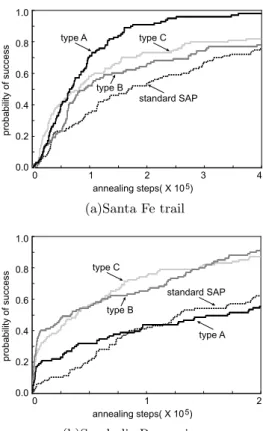
5.2 ^#$

Ö%,±¶

100^s%/q ^§ ^Ô ^q&'t Fig.

4¡2P¯wØz¹Ã¯

Fig. 4^/¯q (a) Santa Fe trail ^î

ï¯ (b)

Symbolic Regression^{î¹ïÇ¡Ã0¯x(}

yxy

$ ²

Fig. 4^)* ^¡ ^§ ^Ô ⁽⁺ ^* ^¡³ ³§t

PwØØ¶$²

Ó³"B

/-,

{ /

t./w

x

Fig. 4«Ä>£Çîï¡£º¶

»¼

´µ

.

´µ«Ä¢

4

§ Ô t

xØ¶$²

Ó³

»¼

´µ

´µo«Ä .yÔ

z³t³s,¬o±

x

±103x

¶¶$

-./01

q 8

¡«yÓ³

'

q

\z

Ä Santa Fe trail^î³ï

"#

1 q t

-.y/0y1

±

¶r²y´yµ

¢}Ó±³¢

«oÂ Symbolic Regression

1.0

0.8

0.6

0.4

0.2

0.00 1 2 3 4 annealing steps( X 10 )⁵

probability of success

type A type C

standard SAP type B

(a)Santa Fe trail

1.0

0.8 0.6

0.4

0.2

0.00 1 2 annealing steps( X 10 )⁵

probability of success

type A type C

standard SAP type B

Fig. 4. Probability of Success.

îï

o

" # 1 q <

Ê³#($te,±$wox /0y1

t

-.y/

0¯1

±¶Ñ²¯´µ

íÇ¢ .

«¯Ó²Ç

¡¯«ÇÄ

-./01

q 8

£îï¡23wx±103x

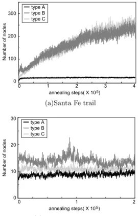
6. ⁴⁵

76

-./01

q 8

¡Ã xÊ#( §q&

'ot Fig. 5^¡Pywz³Ã Fig. 5^/q (a)

Santa Fe trail^îï (b) Symbolic Regression^îï¡¹Ãx

yxy

$ ²

Fig. 5^8)* ^¡yÊ# ⁽ ^§(+ ^* ^¡

§tPw

Fig. 5^«Ä ^$ Santa Fe trail^îï ^{" #} ¹ ^q

t

-y./0y1

±¶$²21"3qyÊ#( §

yx

qm

¡9:,¶$yxq¡£,¶$

' );

q 8

Ê#(

§

(<"=

¡

àá

¶¯x¯

Ç

Santa Fe trail ^î

ï H

yÝ,p$

È è

wxîï

yx²

-

./0y1

t" # 1 t

yÚ

«Ä á z

/01

± 8 wox

±

H

yÝ,p$t

yÚ -./01

t è w

x2&..

4

Â¹z¯x²Ç2¥º±,103Ç

x¯¯q¹²Ç¹

Ê#( § àyá

¶?#%yz " #

1 q t

-y./01

±

8

¶$²´µ

Santa Fe trail ^îï¡Ã

-.

z

(5)

t

²½±=1%3

x

Ø¡ Symbolic Regression^îï

Ø

6´}µ ± ¢Ê #

(ç§

x

qm¡9:'¶

àá

¶?#%yz}

H

Ýo,p$

È è

¶zîï

yx²

±1%3

x

'

¶$q123 " # 1 q <

Ê#($t

e,±$wox /01

t

-.y/01

± 8

¶$²´yµ

í¢

-

.

zt

²±$" # 1 t

Ú

«Ä

á z /

01

¡ -.

¡

Â±=13

x

)

«oÄ SAP^o ^{" #}

1 t

yÚ

«oÄ á z

/y0y1

¡ á

z t=%3x± 0%3x

'

¶$

H

Ý'p$

È è

woxîï

yq /0y1

¡

H

Ý,p$t

Ú

& ¢

à

3xcoÓ³

H

Ý

,p$y

È è

¶zoîï¡³£,¶$

" # 1 q <

Ê³#

($te,±$wox /01

t H

yÝ,p$

È è

wx

îï

" #

1

t

'

-y./01

± 8 wx

± -.

x±103x

300

200

100

0

0 1 2 3 4 annealing steps( X 10 )⁵

Number of nodes

type A type B type C

(a)Santa Fe trail

30

20

10

00 1 2 annealing steps( X 10 )⁵

Number of nodes

type A type B type C

Fig. 5. History of Program Size.

7. ^l

(

SAP^q ^è

µq .0/

±¶

-./01

t $"!Æ¶4ywx´µt

»y¼

¶$² §

»¼ 4 t

²

$

² yÝo,pr

è

wx Santa Fe trail^îï

"#

1 t

-.¯/01

± 8

¶Ñ²¢q

H

¯Ý½pÑ

È è

¶¹z Symbolic Regression

îï

o

" # 1 q <

Ê³#($te,±$wox /0y1

± 8 ¶

²¢q

'

í¢

.Ô

oztwxo±

²«yÓ³£ îïq ¡¤,$

-./01

q

8

tÌ

0

x±

»¼

´µ

«Ä .Ô

z

ts3x±tPw±

²

4

1) J. R Koza, Genetic Programming: On the Pro- gramming of Computers by Means of Natural Se- lection, MIT Press, 1992.

2) , ¹ , ⁽ , ^¾ , ^³!

" #y%&(r)¿*# +³t³²' y³

”, ^â

V W ! "

æ , Vol.48, pp. 88–102, 2007.

3) J. R Koza, Genetic Programming II: Automatic Discovery of Reusable Programs, MIT Press, 1994.

4) T. Asai, K. Abe, S. Kawasoe, H. Arimura, H.

Sakamoto, S. Akikawa, Efficient Substruc- ture Discovery from Large Semistructured Data”, Proc. of the 2nd SIAM Intl. Conf. on Data Min- ing, pp. 158–174, 2002.

5) D.Katagiri, S. Yamada, Speedup of Evolution- ary Behavior Learning with Crossover Depend- ing on the Usage Frequency of a Node”, IEEE International Conference on Systems, Man, and Cybernetics, 1999, No. 5, pp. 601–606, 1999.

6) ^#$%& , ^â^#('æ , ^)*

á

Æ,+ , 2001.

7) N. Metropolis, A. Rosenbluth, M. Rosenbluth, A. Teller, E. Teller, Equation of State Calcu- lation by Fast Computing Machines”, Journ. of Chemical Physics, Vol. 21, pp. 1087–1092, 1953.