Expanded Lyapunov Function for the Transient Stability Problem of a Power System: University of the Ryukyus Repository

Title

Expanded Lyapunov Function for the Transient Stability

_{Problem of a Power System}

Author(s)

Miyagi, Hayao; Taniguchi, Tsuneo

Citation

琉球大学理工学部紀要. 工学篇 = Bulletin of Science &

Engineering Division, University of the Ryukyus.

Engineering(16): 139-152

Issue Date

1978-09-01

URL

http://hdl.handle.net/20.500.12000/27515

JflL球大学理工学部紀要(工学篇)第 16号， 1978年

Expanded Lyapunov Function for the Transient Stahility Prohlem of a Power System Hayao MIYAGド and Tsuneo TANIGUCHI**

Summary

1n this paper， an expanded technique of construction of Lyapunov function is applied to the transient stability problem of a synchronous machine connected to an infinite-busbar. The system model includes velocity governor represented by second-order response. The construction procedure is essentially based on the technique which gives generalized energy function of the similar system. The Lyapunov function is then used to estimate the critical reclosing times. The results are compared with those given by conventional function， and are found to be useful. List of principal symbols 139 M = machine (generator) inertia constant in p. u. power second2 _{per electrical} radian. D =machine damping coefficient in p. u. power-second per electrical radian

ι

ニvoltageproportional to field flux linkage， p. u. E-~i ニ infinite.busbar voltage， p. u. X d = direct axis synchronous reactance， p. u. X" ニquadrature axis synchronous reactance， p. u. X~ ニ direct axis transient reactance， p. u. Xl2ニtotal reactance between the generator terminal and the infinite.busbar， p.u. K" = loop gain of the governing system. T"=equivalent time constant of the governor， s. T_hニtime constant of the prime mover， s. ω

。

=2πん d S - dt 1. Introduction A systematic procedure of constructing Lyapunov functions has been presented previously1)ー :l) for the power system represented by n second.order ordinary Received April 28， 1978 *Dept. of Elec. Eng; Univ. of血eRyukyus 村 Dept of Elec. Eng; Univ. of Osaka Rrefecture

140 Expand_Se_tad_b L_iliy_tya _Ppun_roov_bl F_emu _onc_ft _a ion f_Poor_w t_erh _Se T_ysr_ta_ens_mient

differential equations. The Lyapunov function constructed by the method is equivalent to the generalized energy function of the similar system which is given by multiplying the original system by n-th order real and nonsingular matrix Q. In the process of construction， all elements of this matrix Q are determined so that the curl equations will hold for the resulting energy function and the dissipation funtion will satisfy nonnegatlve property.

More recently， an expanded technique has been developed11日， by considering the fact that the damping force of the system constitutes a energy function. Such energy relates to the dissipation function. In this technique， for the purpose of taking the damping effect into the generalized energy function， the generalized momentum and the potential force are written in some modified forms. The modified form of the momentum includes undetermined matrix αwhich play an important role in the decision of the suitability of the obtained Lyapunov function. In this connection， the modified potential force includes another matrix βdepending onα.

In this paper， an expanded Lyapunov function of a single-machine system is derived， through above-mentioned approach. The system includes velocity governor represented by second-order response.

Then the regions of asymptotic stability for the admissible values of αin the Lyapunov function are examined from a point of view of the critical reclosing time which gives an equivalent estimation of the stability region. Furthermore， it is discussed how the particular matrix αin the Lyapunov function indicates relative offects of control-system parameters on the stability characteristic of a generator 2. Formulation of the problem In this paper， the following assumptions will be made: ( i) field-flux linkages are constant， (ii) damping coefficient is constant， (iii) network is purely reactive Under these assumptions， the swing equation is given by d2_{δ d δ} M一一一十dt₂ D一一一二

Pm-P

ρ ~ dt 川ど ) T Eム ( where

Pe

二

P

1

sin8-P2 s

i

n

2δ p

，

=

E'IE" Xl ~十 Xd p ( x q x;i)E'，f 2 2 (X12十xム)(XI2十Xq)

The variationム

Pm

in power input to the synchronous machine owing to the action of a governorcl is

琉 球 大 学 理 工 学 部 紀 要 (工学篇)第16号.1978年 141 ムPm二 kgiEL-

一一一_

1 川島 ωo(1

+

Tgs)(1 +Ths) (2) Definingnew variables as X1=δδo X2=ムPm X3=( 1

+

ThS)xZ we can represent thesystemin the following form (3) 、_{1 1} 1 1 E 1 1 1 1 1 1 1 1 1 ノ ハ U A U A U 〆 t 1 1 1 1 1 1 1 E 1 1 ﹄ l l t_、 一 = 一 、_•••• ' ι ' a . . _、 r E ‘ ' P a 目 目 目 目 1 l l l l ￨ 1 1 l ι 1 i l I J )

x

o

o

( g f l 1 t i t i l

-、

自 ￨ 制 ￨ 川 叩 n u n υ n り わ 0 0 〆 l l f ﹄ 1 1 1 1 1 1 h t l_、 十

、

I I B i l l i -J 1 2 3

x

x

x

fIlli--L

、

l i l l 1 1 1 1 J

o

寸 ん 2 1 ; η ! Y 1 A U A U A り 〆 l l ﹄ l I P E t t i --_、 ， ， E E ‘ ， E E E ， ︿ ‘ E E E B E E B_{‘ 、}

+

、₁ l h 1 1 1 1 1 1 1 1 f l l ノ 1 2 3 ・

x

・

x

x

r i l l l 1 1 1 1 1_、 、f_l l g l a z i -1 l ノ ハ U A U ' i A H U 唱_E A A H υ 、 A n 小 O -f i l l -1 1 1 1 1 1 E_{， 、}

+

、

_{B I} B I -1 -1 E E E ' l l ノ 1 1 1 2 1 3 & X 十 ん 土 〆 l l ﹄ 1 1 1 6 1 B ﹃ l l t _、

、

l i li----J n υ ハリハリ ハ U A H V A H V 1 A A U A U r I l l i -I l l -

、

(4) where

D

1 ，P 7}1=M' 甲2 -肩. 7}3= M' A.

=

_

_

!

i

c

_

ー

ん

=_1_ .ω

。

T_K ' '" T_g' PO=P1sinoo-Pzsin 2δ

。

山 1)二 川(X1+δ0)

含

sin2(Xl+δ0)

昔

3. Expanded Lyapunov function For thebrief description， eqn.(4)is rewrittenin the form Mx+ Dx+f(x)=O (5) where

ピ

=(X1X2 X3)

。

。

1

D=[:

。

。

_o

D.1 =I 0

。

OJ L-A.

。

l

L

(

X

)

i

f(x)=1 !z(x)

!

，

(x) 1 1 1 I l l i -J D 川 一 D U 然 ハ リ 十 z x g 2 1 Illi--ー ノ 刀 0 0 0 . げ 0 0 0 0 ρ 一 P -A り A U 、 / Y 4 0 〆 I l l 1 1 1_L m O

+

+

z i λ

、

l_t B E ﹃ ' E E ' t i l t / 〆 f k ) れ 2 n ( 一 A 幻 〆 l t i t i -F I ﹄ P ﹄ } l l 也、 一 一 わ れ o n 1 I l l l ノ

。 。

付

o o 〆 l i l i --

、

g = r ill--ー に 一 一

z

g Considering3 x 3 nonsingularmatrixQ as

142 Expand_Ste_ad_bilL_iy_ty apu_Pn_ro_obv F_lemu _onc_ftio_a n f_Powor t_er he T_Sysr_ta_en_msient 1(/11

，

/

(

"

(/l:l I

Q

=

I

(

/

"

'

(/"， ピ1"l

I

l(/':I ({，，， (/:n) ) ) ( [ the similar system obtained by multiplying bothmembersofeqn. (5) byQ becomes Hi:+R土+G(x)二

o

(7) where H二 QM. R=Q D G(x)二 Qf(x) Introducing undetermined3 x 3 matricesα and β， system (7) ismodified as follows:

-

_rl

~(H.i:

_l

+

H α Rx

)

+

(I-H α

)

Rx

十〔βx十G(.r))=βz 山 口 where， 1 shows 3 x 3 unit matrix

From eqn. (8)， the generalized momentum P (x， x) and the generalized

potential forceF (x)appear as P(x. :i:)=H x十HαRx F(x)二 βx+G(x) ) ) 、 7 0 4 l ( ( For a line integral ofeqn. (9) tobe independent ofthe path ofintegration， we obtain (h l

=

{/:ll二 O ) -l ( Moreover， foreqn. (10)， therelationships β=β7 命) /u l ( {hl二 {/:ll二

o

わ -__L!_，. 一一___!b_川 三 二 一一-(/，，， (/l:l一 、 (/"一 、 q 1I 1¥， 1¥ ( l -) 似 r二

f

す十「戸((/川/ areobtained asc

∞

on叶d出凶1比tio凶n1渇st出ha討tthe potential energyi応sum悶qu凹1児elydetermined. Eqn. (12)

shows βmust be a symmetric matrix.

From eqns. (11) and (13)， Q becomes ({I 1 II') ーーナ-(/11 r 1

f

ケ

qll

。

ニ

I0 _q"

ラ

ケ(

_q

_，

_"

_{川 )} ( 1 4 )

o

{/:." q:u In orderforQ tobe nonsingular， theconditions (/1 1宇

o

Jhi球 大 学 理 工 学 部 紀 要 (工学主主)第16号.1978年 143

({22(!:n

寸

ケ

(

{

:

l

2(({'2+ 恥 )

must besatisfied.

Now， using eqns. (9) and (10)， the Lyapunov functionV is given by

V(x. x)二

.

f

o

x[p(x. x))rdx+

o

!

x (F(x)JIdx ( 15) T A 、_目1 1 4 E Y R ほ

α

口 、

+

α

い_は H H I α ? 剖

R

V

R 一 リ α β Z 十 ( ( ・₃ 1 2 G 1 れ [ 十 Z I l l .

-

_一

2 9 j h 二 十 (16) with . ¥I(x， i:)三一ど((l

-

H

α

)

R

)

r

.

ーピ

(Rf_{αfRβ)x一〔αRX)TG(X)} ( n， l ，) To begin with， considering theconditionswhich ensurethe positive definiteness ofV shown ineqn. (16)， the relations ハ U > 一 n H n β o 一 >

R

Z

a J U

H

r

d

z

T J t

o

z

G

> -J i z ︹ H 仕

f

l

A

(n=aR) ( 18) ( 19) (20) are glven. Relation (15) and inequality(18) lead to ({，，> 0 The conditiongivenby inequality(20) yields ({，，> 0

I

(/22> () r q22(._l'({:l2十

A

，({日)-l' (1~2

>

0

J Next， under considering the semidefinitenessofV are S 二~ 0 Rf_αfR-β=0 xT(αR)TG(X)'20 ) n r “ 2 ( above relations， theconditionsof the negative (23) (24) (25)

where， S indicates symmetric portion ofmatrix(1-Hα)， R.Eqn. (24)shows αbecomes

a symmetric matrix. Considering eqn.(24)、inequality (25) gives the following three relationships

n

"

ミ

o

I n'2二 flt:l=fl2F n:ll = 0 f n 22({22十 的2q泊三

o )

) μ h u n ソ F M (

144 ExpandSetadb Liliytay Ppunroovbl Femu oncft a Power Sion for the Tysrtanesmient where n=αR 1 nll n12 n13I 二￨刀21 n22 n231 l .n:ll n32 n33) ) 7 2 (

From eQns. (24)and凶， we obtain

n22=

K

2

寸

)q33-q

J

2

}

山 Y1 L1 n

一旦

d竺二71q22)平2n11qll 23- YlL1 n) X 0 9 ' u ( η

一

一

{Ylq22

+

(Yl

+

，12)q

2

J

}

甲2nllq1l 32- Yl L1 nn=-_{33一一 一 .}_!j_2 n11 q32 q11 where， L1=，1

1

{

q22(山 +，1

2

q33) -Ylq

;

k

}

>

0 Using the relation n=αR and eQn.(28)， following ineQualities are derived : n11ニ ザ1α11qll二三 O (29) nラ IAヲ I q22n22十q32n32=

ー

_y1

ム

_，1l'ニ+11 1¥ Yl' 4 J

where α11is a element of 1・st row and l-st column of matrix α.

Moreover， following rearrangement can be done :

i:

T

S

土 =(土l h〕

(

B

4

5

)

[

;

;

]

十q33(お

+

(

X

I

，X2J

去

r

(30) where

、

BI

、

3 4 B P ' q 十 月 u_・

:

!

、

_μ ' V ' ' 一 2 2 1 τ A 3 、 A 一 η 一

一

+

わ 一 2 仏 、ん一九わ一れ 一 ， E l d -- _、 け 1 一 2 h 川 ↑ f tE ﹄ E l l -﹄ I 1 1 1 1 1 1_、

一

一

B

計

三

q

←

)

J

1

l

-

f

(

た

q

十

士{

q32+

た

(q川

2

3

)

}

I

琉球大学理工学部紀要(工学篇)第 16号， 1978年 145 Ifthe relation B-坐

f

q33 ) -q 喝 U ( is used， eqn. (30) is given by a perfect square expression. Then， inequality q33> 0 (32) guarantees that the matrixS becomes positive semidefinite. Eqn. (31) yields following three equations: 2 、 、 、 ‘ . ， ， ， ， ， 3 3

q

、 パ十 月 w a わ 一 ん J ' t ' t_、 、 一 一 3 3 G A G a 、 、 、 EE ﹄ ， F 5 5 5 ' 制 H 2 2 ん 一 A

+

n " ' ， ， s a_{‘ 、 、 、} a 斗 ゐ ) 3 q 喝 d (

2

(

r

q

1

1

十 ぞ ( 伽

+

q32)}q33

=

(

Z

q

川 1

寸た(耐仇

2)+白 ) 4 n d d ( 4 ω 3

戸

=

イ

(

去

(

q

耐伽

ω)

汁+汁

伽

叩q

仇

切3泣2 Solving the above equations， we have (35) q33=fqll q22= mqll (36) q32= nqll and f =

会

{

(

2

711ー 2nll

十

4

7

2

)

:t

2

ん-

nll)(711-nl1

十

台

子

)

}

>

0 m =

会

{

(

2日 1h2):t2

.

j

C(f-h1 h2) }

>

0 n =

ー

す

(

た

(

た

-

川m

-

2

6

r

)

h

1

=

者

ベ

l

f

)

- 一 γ ' 一 j ↑ A y

t

一 ん q L 一 9 3 “ h

ρ

ニ

(

た

+t1

1

f

)

(

1

+

た

)

-

2 t11

会

Here， as the valuesf and m must be real and positive， the following relation is obtained by using eqns. (22) and (33):

146 Expand_Se_tad_b L_iliy_tya _Ppun_ro_ov_bl F_emun _oct_{f a} ion f_Poor_w t_erh _Se T_ysr_ta_ens_mient

O:S:n

匂点目前

:

i

j

i

J

1

7

i

j

n

The above expression will impose certain restrictions on the control system parameters

K

.

q

and

T

q

for the variousnll・ N ow， the Lyapunov functionV becomes (37)

r

1 . 0 1 叩11

V

(

ι

i')ニ qlll_{L 2 ' 2"} ~ X12→(止l+nll_..X_.1)2+ ー(甲l~nll)xi'_{. 2} 、 ， E 与 S E a p x

、

、

l i l 1 1 1 / ρ ε 一 ρ ε 、 d ハ 一 、 d 八 十 一 一 わ 一 ん 一 柄 引 一 ん / ， s t i l l i -t ¥ ん 一 れ 十

x

x

〆E B E g -E E t、 、ltr ・ -E F

、 、

l s ' / n u 令 、 パ わ 一 ん 〆 ， ， E E t

、 、

2 1 一 A Y Y 一 ん 〆 E l t E E_{， 、} m 一 2

+

+μ ()..2P~

2

ゎ ル

、_{E B} E t h 4 1 1 F 。 U ヘ ハ υ 十 X Q U A v f し o m O ︽ U o f し / l l イ I1 1 3 η ' 十 X 3 円 γ 九 一

R

ヰ

:

ト

os

2δO~

cos2 ( 川 ( 3 OXυ) with

V(x

， .t)

=

~

q

l

J

[

市

-

C

+

7

3

2

去

)

X

1

+

(

先

7

7

i

;

血す

_

2

ゐ

)

r

← f1 (n22X2 +η23X3)( mX2+ηX3) (n32X2

+

n33X3){ f1 n (X2

~

X3)

+

)..2i'X3} 十TJ3n

J

l

X

い

(

円

。

)-25in2(け 0)~

~:}J

Then， the critical value of the Lyapunov function is given by (39)

院。「 η(

!l_l_十)..1TJ2

し

2

旦

_{η x} ← ぜ

I

J

l

"

1

J

¥

2 I 2 )..2)"IC _P 1" ん 十甲

3

{

ω

δ

o

州 X1C十 品

H

全

(

川

an AHV ) t ( where X1Cimplies the unstable equilibrium state ofXJ， cIosest to the stable equiIibrium state.Itis found that eqn. (40) has no connection with i'and m. On the other hand，

V shown in eqn. (38) depends on these values.Ifone choosesi'and m so that V has the minimum value in any solution trajectory， a wide range of asymptotic stability can be obtained.

琉球大学理工学部紀要(工学篇)第16号.1978年 147 In the results， a suitable Lyapunov function will be given choosing

p=剖~

2 T}l-2 nll

十

ぞ

)-

2

j

T}l -nll)(早l-nll+

ぞ

)

}

m =

す{(

2 P -h 1 h2 ) - 2

，，(l(l司お)

) 1 4 ( (42) η ニ_l~旦{笠 -ÀIP)m ← 2jfj_2.~

ρ

l

A

2

¥A2 且

r

-vytJ Using eqn. (29)， Vc given in eqn. (40) is rewritten in the form ) n 4 J V 4 (

「

αllD'2..2 PO_ ，Pd ~~~" ~~~(_

，

"

J

Vcニ qIll-EEEXlc-EXIC+

副

COSδ0 -COS(XIC十δ

0

)

)

長

ト

os2ゐ-COS2附 a n宮4 ) ( where D'ニイD(D+l(

q

/

'

ω。) Since inequaIity D'>D

。

句

is existed， it is shown that the gain of the governing system contributes to reinforcing of damping of the generator.l5 4. Application to the transient stability problem The following numerical examples are presented to investigate the stability region of the expanded Lyapunov function. Consider the system as shown in Fig. l. The generator is connected to an infinite bus through a double transmission line. The values of the svstem parameters are given in Table l. A symmetrical three phase fault to ground is assumed at point F in Fig. l. The faulted line is disconnected after 0.1 second and is reclosed subsequent to time to・ Thecritical reclosing time r c [ニ0.1+ t 0 J. in which the system will return to a stable state， is determined by using the Lyapunov method， and is then compared with that obtained by numerical integration. The critical reclosing times are obtained for the variousn l1/nm(ニ甲1q日al1/nm).

Fig.2 shows cross-sections of stability boundaries in the planex2=0.075 and X 3 二 0.09 for the admissible values of nll/η刑 . The parameters are given as Kg=20，九 二 0.1 and T_hニ0.5. The line section between 0 and B shows trajectory under fault， and the fault has been cleared at point B. Although these figures are only the projections on (x1， Xl) space， the effect ofα11 on stability boundary may be illustrated.

148 ExpandSteadb Lilfytya -puPnroovb Flemu oncft a ion jPoorw terh Se_ Tysrtaensmient K.

I

Llω I (1 +ThS)(1 +T.slω。 V

，

F Fig. 1 Diagram ofsystem studied Table 1. System constants X d = l.0 XI2 =1.12 M =0.0138 0 0 Xq =0.6 E~ =l.208 X1 B X

d

=0.4 EH =l.0 1.0 Fig.2 Regions of asymptotic stability E" 1111/l1m = 1 111

，

/n.o=0.5 111，/l1mニ O 2.0 X

，

X2 =0.075 X

，

=0.09 T. =0.1 T" =0.5 κ.=20

琉球大学理工学部紀要(工学篇)第16号，1978年 ₁₄₉

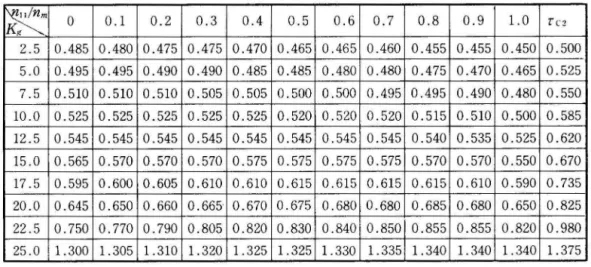
Next， the critical reclosing times for the various system conditions obtained by varyingKg are computed. The results for the admissible values ofn 111 nm are given in Table 2， comparing with the results obtained by step by step method. Table

shows that the useful Lyapunov function， in thesense of giving wide stability

region， varies in accordance with system condition.

Furthermore thecontrolsystem parameters Kg and Tg are restricted by eqn. (37). Figs. 3-9give such restrictions for the variousn ul仇(=q uau)' These results

show thatthemagnitude ofdamping coefficientallows wide range ofn ul1Jl・

table 2 Critical reclosing times forvariousn111 n.

除

ぞ

m

。

0.1 0.2 0.3 0.4 0.5 0.6 0.7 0.8 0.9 1.0 fC2 2.5 0.485 0.480 0.475 0.475 0.470 0.465 0.465 0.460 0.455 0.455 0.450 0.500 5.0 0.495 0.495 0.490 0.490 0.485 0.485 0.480 0.480 0.475 0.470 0.465 0.525 7.5 0.5100.5100.5100.5050.505 0.500 0.500 0.4950.4950.4900.4800.550 10.0 0.525 0.525 0.525 0.525 0.525 0.520 0.520 0.520 0.515 0.510 0.500 0.585 12.5 0.545 0.545 0.545 0.545 0.545 0.545 0.545 0.545 0.540 0.535 0.525 0.620 15.0 0.565 0.570 0.570 0.570 0.575 0.575 0.575 0.575 0.570 0.570 0.550 0.670 17.5 0.5950.6000.6050.6100.610 0.6150.6150.615 0.615 0.610 0.590 0.735 20.0 0.645 0.650 0.660 0.665 0.670 0.675 0.680 0.680 0.685 0.680 0.650 0.825 22.5 0.750 0.770 0.790 0.805 0.820 0.830 0.840 0.850 0.855 0.855 0.820 0.980 25.0 1.3001.3051.3101.320 1.325 1.325 1.330 1.335 1.340 1.340 1.3401.375 nm : maximum valveof nl1

九=

0.1 (sec) Th = 0.5(sec)δ

。

=40(deg) 5. Conclusion

Using the expanded technique， Lyapunov functionis constructed in a systematic way for thetransient stabilityproblem. The featurewhich distinguishes the method

isthat the damping effect is taken into the generalized energy function ofthe similar system. For a synchronousmachine swinging against an infinite-busbar， including governor effect representedby second-orderresponse， a setofLyapunov functionis constructed. As a Lyapunov function which gives better estimation varies in accordance with system condition， theboundary ofthe unionofthesuitableregions may beusedin the practical study. The application to the system with automatic voltage regulator is being currentlyinvestigated

Expanded Lyapunov Function for the Transient

StabilityProbJem of a Power System

Kg=15

s

bo h 1.5 1.0 0.5 均 =20 150 u お bo い 2.0 1.0 0.5 1.5 1.0 1.5 11， 1r， ;; 0.5

。

0.5

。

1.5 I1IfI ;rI Domain nf of宿 (Kg=lO) 1.0 Fig.3 Domain of宮 (Kg=15) Tg = 1 .O(sec) Fig.4 h ~ 40 Kg=20 u o c -H Q u お

'

"

い 2.0 1.5 0.5 1.0 1.0 11" I，;r Tg (Kg=30) 0.5 Domain of Fig.6 1.5 11，，17)I Tg (Kg=20) 1.0 Dorr】ainof Fig.5

。

琉球大学理工学部紀要(工学篇)第16号， 1978年 u g 向 2.0 1.5 1.0 0.5

。

一_-.一一一・一一r γー一 -1.0 1.5 Il，，/T}I Fig.7 Domain ofKg (lg=O.I) 40

"

"

~ 30 _Tg=0.4(sec) 10

」一一一-

一

一

"

"

~ 30 持=O.l(s氏) 20 凸 U I

。

0.5 1.0 Illl/T}I Fig. 8 Domain ofKg (1云=0.4) 1.0 nll/T}I Fig. 9 Domain ofKg (在=1.0) 151

152 Expand_Se_tad_bilL_ity_yapu_Pn_ro_obv F_lemunc_oft _a ion_Pf_oor_wet_rh _Se T_ysr_ta_ens_mient

Acknowledgment

The authors acknowledge Mr. Y. Umano， Mr. K. Kakihana and Mr. Y.

Sawamori， students of UniversityofOsaka Prefecture， fortheirassistanceofnumerical

calculation.

References

1 Tsuneo Taniguchi and Hayao Miyagi : 'AMethod of ConstructingLyapunov

Functionsfor Power Systems'， Trans.ofIEE of]apan， 1977， Vol.97.B， No. 5，

pp.271-278

2 Hayao Miyagi and Tsuneo Taniguchi 'Construction of Lyapunov functionfor

power systems'， Proc. IEE， 1977， Vol.124， No.12， pp.1197-1202

3 Hayao Miyagi and Tsuneo Taniguchi 'Transient StabilityRegionsof Power

Systems'， BulletinofScience& EngineeringDivision， University oftheRyukyus，

1978， Eng. No. 15， pp.. 105-114

4 Tsuneo Taniguchi and Hayao Miyagi 'AMethod of ConstructingLyapunov

Functionsfor Power System basedon theEnergy Concep'，t Trans. ofIEE of

] apan， 1977， Vol.97・B，No.2， pp.l07

5 Tsuneo Taniguchi 'AMethod of Constructinga GeneralizedLyapunov Function