PAPER
Special Section on Wideband SystemsDiversity Reception and Interference Cancellation for Receivers Using Antenna with Periodically Variable Antenna Pattern
Nobuhide KINJO†,Nonmember andMasato SAITO†a),Senior Member
SUMMARY In this paper, we propose a model of a diversity receiver which uses an antenna whose antenna pattern can periodically change. We also propose a minimum mean square error (MMSE) based interference cancellation method of the receiver which, in principle, can suffer from the interference in neighboring frequency bands. Since the antenna pat- tern changes according to the sum of sinusoidal waveforms with different frequencies, the received signals are received at the carrier frequency and the frequencies shifted from the carrier frequency by the frequency of the sinusoidal waveforms. The proposed diversity scheme combines the com- ponents in the frequency domain to maximize the signal-to-noise power ratio (SNR) and to maximize the diversity gain. We confirm that the bit error rate (BER) of the proposed receiver can be improved by increase in the number of arrival paths resulting in obtaining path diversity gain. We also confirm that the proposed MMSE based interference canceller works well when interference signals exist and achieves better BER performances than the conventional diversity receiver with maximum ratio combining.
key words: space diversity, path diversity, ESPAR antenna, MMSE, inter- ference cancellation
1. Introduction
Space diversity techniques are effective measures to im- prove the receiving performance in a multipath fading en- vironment of wireless communications. Although the in- crease in the number of receive antennas improves receiving performances, the resulting antenna sizes can be a problem because the antennas need separation more than a half wave- length.
To solve the problem, several diversity receivers have been proposed using electronically steerable passive array radiator (ESPAR) antenna whose antenna patterns or di- rectivity would be periodically changed for single-input multiple-output (SIMO) and multiple-input multiple-output (MIMO) receivers[1]–[9]. ESPAR antenna consists of an active element and several parasitic elements [10]. Since the parasitic elements are terminated by variable reactance (VR) elements, we can change the antenna pattern by chang- ing applied voltage to the VR elements. In the previous work mentioned above, they use a sinusoidal voltages to periodi- cally change the antenna pattern in sinusoidal manner. The sinusoidal antenna pattern can generate diversity branches in the frequency domain (See Fig. 1 in Sect. 2).
When we use such an antenna, it is natural to select the amount of frequency-shift (shown as fsin Fig. 1) so that
Manuscript received April 10, 2020.
Manuscript revised August 7, 2020.
†The authors are with University of the Ryukyus, Okinawa- ken, 903-0213 Japan.
a) E-mail: masato [email protected] DOI: 10.1587/transfun.2020WBP0006
parts of desired signal is shifted to the frequencies vacant or not used during reception. However, if we fail to find vacant frequencies, the undesired signals may exist at the frequen- cies to be shifted. In such cases, since both the desired and undesired signals are frequency-shifted by the same amount due to the property of the antenna, they can be interfered with each other (See Fig. 3 in Sect. 3 and Fig. 8 in Sect. 4.2).
In this study, we call the undesired signals uniquely caused by periodically variable antenna pattern interfering in the desired signal interference.
Although general array antennas could realize the an- tenna with periodically variable antenna pattern (PVAP an- tenna), there are several disadvantages. Firstly, the number of diversity branches built by array antennas is less than that done by ESPAR antennas. Due to the linearity between an- tenna input and output signals, array antennas are difficult to build useful diversity branches more than the number of antenna elements[11]. On the other hand, ESPAR antennas can construct the number of diversity branches more than the number of antenna elements due to the nonlinear char- acteristics between the applied voltage to VR elements and antenna patterns[12]. Secondly, it might be difficult to re- alize high-speed phase switching or have limitation to the speed. Although it depends on the characteristics of VR ele- ments, we experimentally confirmed that ESPAR antennas can change their antenna patterns with more than a hun- dred MHz [13]. Thirdly, the size of array antennas is rel- atively larger than that of ESPAR antennas. While array antennas need more than a half wavelength between neigh- boring antenna elements, the separation between an active element and parasitic elements of ESPAR antennas should be less than a quarter wavelength. Since ESPAR antenna utilizes mutual coupling between antenna elements, the ar- ray antenna can be relatively larger size than that of ESPAR antenna. Finally, cabling cost is large in the case of array antennas. The array antennas need the number of cables connecting antenna elements to the receiver is equal to the number of antenna elements. On the other hand, ESPAR antenna only needs one cable which connects the active el- ement and the receiver. Due to the reasons above, ESPAR antennas are the first candidate to realize PVAP antennas.
In this study, we propose a diversity reception scheme for receivers using antenna with periodically variable an- tenna pattern. Moreover, we study the cases that there exists an interference signal in a frequency-shifted component and there exist multiple interference signals in frequency-shifted components. To reduce the effects from interference signals, Copyright c2021 The Institute of Electronics, Information and Communication Engineers
a single and double interference signals in the neighboring frequency bands.
This paper is organized as following. In Sect. 2, the system model is illustrated. Section 3 explains the pro- posed diversity receiver and interference canceller. Then, in Sect. 4, numerical results obtained by computer simulation are provided to evaluate the BER performances obtained by the proposed receiver. Finally, Sect. 5 concludes this study.
2. System Model
In this section, first, we describe the receiving process of the receiver with an antenna with periodically variable antenna pattern (PVAP antenna). Then, we propose a system model of the diversity receiver with PVAP antenna. The PVAP an- tenna can be realized by ESPAR antenna[1],[6],[8],[14].
In general, ESPAR antenna consists of an active antenna el- ement and multiple passive antenna elements. The passive elements are terminated by VR elements[10],[15]. To the multiple VR elements, if we apply a combination of con- stant voltages, we can arrange the antenna beam pattern ac- cording to the combination[10]. Instead of those constant voltages, periodical voltages, for example, sinusoidal volt- ages can be applied to the elements in order to change the antenna pattern in a periodic manner[8],[16],[17].
In this study, we focus on periodically varying the an- tenna patterns of ESPAR antennas. We build a time-variable antenna pattern model of the PVAP antenna. The ESPAR antenna considered here has Npe parasitic elements. Sup- pose that we apply the following DC biased sinusoidal volt- age to the VR element of thek-th parasitic element of the antenna fork=1, . . . ,Npe.
vk(t)=V0,k+V1,kcos ωst+θ0,k (1) whereV0,kis DC voltage,V1,kis the amplitude of sinusoidal component,ωs is an angular frequency common to all the VR elements, andθ0,k is the initial phase of the sinusoidal component. The voltages can change the reactance of each parasitic element, then the change of reactance can vary the antenna pattern or directivity of the antenna. Since the re- lation between applied voltage waveforms and the obtained antenna patterns are nonlinear, the antenna patterns can have harmonic components ofωs. However, we found experi- mentally that such harmonics could be relatively weak com- pared with the components of DC and the fundamental fre- quencies±ωs[16]. Therefore, we assume the following an-
tics of VR elements, applied waveforms (1), azimuth, and so forth.
When a receive antenna receives a signal from a direc- tion, the antenna output can be mathematically shown as the product of the received signal and the antenna pattern for the direction. Suppose that a signal coming from a directionφ can be given asr(φ,t). If we use the antenna whose antenna pattern is given by (2), the baseband antenna outputy(φ,t) can be shown as follows.
y(φ,t)=r(φ,t)D(φ,t) (3)
=r(φ,t)D−1(φ) e−jωst +r(φ,t)D0(φ)
+r(φ,t)D1(φ) ejωst. (4) In the right-hand member of (4), each term can be orthog- onal to each other, ifωsis sufficiently large. Hereafter, we assume thatωsis large enough to keep the orthogonality be- tween the received signal components in the frequency re- gion. Considering the orthogonality, we can write (4) in the following equivalent vector form.
y−1(φ,t) y0(φ,t) y1(φ,t)
=
D−1(φ)
D0(φ) D1(φ)
r(φ,t) (5)
whereyk(φ,t) fork=−1,0,1 are the received signal com- ponents at the frequencies ofkωs. We defineNras the num- ber of orthogonal components of the received signals (5).
The number can be also recognized as the number of receive diversity branches. In the case of (5),Nr =3.
In multipath fading environments, received signals or elementary waves could come from multiple directions.
Therefore, when Np signals from the directions of φk for k=1, . . . ,Nparrive at the receiver, the antenna output in the vector form can be shown as
y=
y−1(t)
y0(t) y1(t)
=
Np
X
k=1
D−1(φk) D0(φk) D1(φk)
r(φk,t) (6)
=Dr, (7)
where D is the Nr ×Np matrix including antenna pattern coefficients which is given as
D=
D−1(φ1) D−1(φ2) · · · D−1
φNp D0(φ1) D0(φ2) · · · D0
φNp D1(φ1) D1(φ2) · · · D1
φNp
, (8)
Fig. 1 Spectra of (a) transmitted signal or input signal to the received antenna, (b) received signal received by general antennas, and (c) received signal received by PVAP antenna.
andris the vector of received signals shown as r=h
r(φ1,t) r(φ2,t) · · · r φNp,tiT
, (9)
whereT is a transpose operator. Hereafter, we refer to D andras antenna pattern matrix and received signal vector, respectively. As a visualized reference, in Fig. 1, we illus- trate the spectra of (a) a transmitted signal or equivalently an input signal to the received antennas, (b) a received sig- nal received by general antennas, and (c) a received signal received by the PVAP antenna whose antenna patterns are given in (2). Here, we assume the carrier frequency of the transmitted signal is fcas shown in Fig. 1(a). As shown in Fig. 1(c), the antenna pattern generates three received sig- nal components in the frequency domain at the frequencies fc− fs, fc, and fc+ fs, where fs =ωs/2π. After frequency conversion to baseband, the components at fc− fs, fc, and
fc+fsin Fig. 1(c) can be written as (7).
Instead of (1), if we consider a DC component and (Nr−1)/2 orthogonal sinusoidal voltages, we can generalize the antenna pattern as
D(φ,t)=
(Nr−1)/2
X
k=−(Nr−1)/2
Dk(φ) ejkωst. (10) As with the case ofNr = 3 shown in (2), we assume that for a given number of orthogonal sinusoidal voltages the ef- fects of harmonic components can be ignored to generate onlyNrorthogonal components as shown in (10). Then, the corresponding antenna pattern matrix to (10) is given forNp arrival paths as
D=
D−(Nr−1)/2(φ1) · · · D−(Nr−1)/2 φNp
... ... ...
D0(φ1) · · · D0
φNp
... ... ...
D(Nr−1)/2(φ1) · · · D(Nr−1)/2 φNp
. (11)
Since the symmetry of the frequencieskωs,Nrshould be an
Fig. 2 System model including the receiver with PVAP antenna (Nr=3).
odd number.
Based on the receiving process mentioned above, we describe the system model of the receiver with PVAP anten- nas. The proposed model is shown in Fig. 2. The transmit- ter sends a complex symbol sto the receiver through mul- tipath fading channel. The average power of sis assumed Eh
|s|2i
=1, where E [·] is an averaging operator giving the average value of the argument. The carrier frequency is fc.
The number of arrival paths at the receive antenna is Np. Each path experiences fading effects, then the path com- ing from a directionφkis multiplied by a complex channel coefficienthk. Since we assume Rayleigh fading channel throughout this paper, the coefficient hk can be a complex Gaussian random variable with the mean E [hk]=0 and the mean square Eh
|hk|2i
=1.
The arrival signal coming from the directionφkcan be shown as
rk=hks. (12)
WhenNppaths arrive at the antenna, all the arrival paths can be given in a vector form as
r=hs, (13)
wherehis a vector of channel coefficients and is defined as h=h
h1 h2 · · · hNp
iT
. (14)
Note that the carrier frequency of each path in (13) is fcbut not fc±fs. As shown in Fig. 2, the components atfc±fsare generated inside the antenna but not during propagation.
Substituting (13) into (7) and considering additive white Gaussian noise (AWGN) in the channel, we have the antenna outputs in a vector formy∈CNr×1as
y=Dr+n=Dhs+n (15)
wheren∈CNr×1is the noise vector defined as
In this section, we propose a diversity receiver with the PVAP antenna. Then, we consider the case of existing in- terference signals in the neighboring frequencies. After that we propose an interference canceler for the receiver based on MMSE criteria.
First, we discuss the behavior of the interference sig- nals when PVAP antenna is used at the receiver. The spectra of the received signals, which are desired and interference, are shown in Fig. 3. Figure 3(a) and Fig. 3(b) show the spec- tra of the antenna inputs and outputs, respectively. Here, the carrier frequency of the desired signal is fc. As is the case in Fig. 1, the desired signal can be frequency-shifted by±fs
according to the antenna property and appeared at not only fc, but also fc± fs, as shown in Fig. 3(b). When the carrier frequencies of fc−fsandfc+fsare used by other transmit- ters, their transmitted signals can be interference signals. If two interference signals are sent with their carrier frequen- cies of fc±fs, the received signals also suffer from the an- tenna property. Therefore, the property makes the desired as well as interference signals frequency-shift by±fs. As can be seen from Fig. 3(b), any signal appears at its carrier frequency as well as its neighboring frequencies due to the property of PVAP antenna. Therefore, if there are interfer- ence signals at either or both offc−fsandfc+fs, the desired signal components at fcand fc±fssuffer from the interfer- ence.
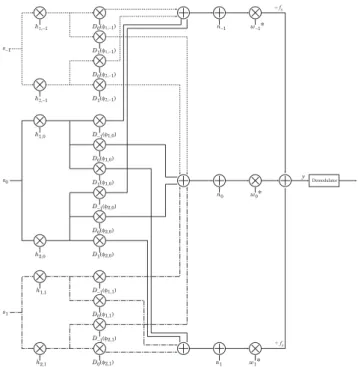
Then, we describe the system model of the proposed di- versity receiver with interference signals. The system model is shown for the number of arrival paths Np = 2 and the number of diversity branchesNr=3 in Fig. 4.
We assume that the carrier frequencies of the desired signal s0 is fc. We also assume two interference signals s−1 ands1are centered at fc− fsand fc+fs, respectively.
The receiver can selectωs. It is natural to avoid interference signals when selecting the angular frequencyωs. However, here, we consider a relatively severe case for receiving de- sired signal in terms of interference. The power of signals are normalized as Eh
|sk|2i
=1 fork =−1,0,1. Using the receiving process discussed in the previous section, we have the antenna outputsyin the vector form as
y=D−1h−1 s−1
√γ−1
+D0h0s0+D1h1 s1
√γ1
+n, (17) whereγkfor (k=−1,1) is signal-to-interference power ra- tio (SIR), the power ratio of the desired signal to the interfer-
Fig. 3 Spectra of received signals at the antenna inputs and outputs with interference signals in the neighboring frequencies.
Fig. 4 System model of the proposed diversity receiver with interference signals (Np=2,Nr=3).
ence signals atfc+k fs,hkandDkare the channel coefficients vector and the antenna pattern matrix for sk, respectively.
The channel coefficients vectorhkis given as hk=h
h1,k h2,k hNp,kiT
. (18)
Considering the overlap between signals (see Fig. 3(b)), we can write the antenna matricesD−1,D0, andD1as
D−1=
D0 φ1,−1 · · · D0
φNp,−1 D1 φ1,−1 · · · D1
φNp,−1
0 · · · 0
, (19)
D0=
D−1 φ1,0 · · · D−1
φNp,0 D0 φ1,0 · · · D0
φNp,0 D1 φ1,0 · · · D1
φNp,0
, (20)
and
D1=
0 · · · 0
D−1 φ1,1 · · · D−1
φNp,1 D0 φ1,1 · · · D0
φNp,1
, (21)
respectively. The third row of (19) corresponds to the an- tenna pattern coefficients for the frequency band centered at fc−2fs. Since the frequency band should not include the desired signals in this model, we set zeros the row to ignore the components in the frequency band. For the same reason, the first row of (21) is also a zero vector.
The antenna output (17) is multiplied by the Hermitian transpose of a weight vectorw∈CNr×1. The weight vector wis given as
w=h
w−1 w0 w1i
. (22)
In Fig. 4,∗means a complex conjugate operator. Hence, the decision variablezfor demodulation can be given as
z=wHy, (23)
whereH is a Hermitian transpose operator. In this study, we determine the weight vectorwaccording to MMSE cri- teria[18]. We define an objective functionJ as the mean square error between the decision variablezand the desired signals0[19]. Then, the functionJis given as
J=Eh
|z−s0|2i
(24)
=E
wHy−s0
2
. (25)
The weight vectorwwhich minimizes (25) can be obtained through a mathematical manipulation given in Appendix in detail, as
w= 1
γ−1R−1+R0+ 1
γ1R1+2σ2INr
!−1
E [D0h0]. (26) whereRi is the autocorrelation matrix of the vector Dihi, we refer to this vector as equivalent channel vector, 1/2σ2 means signal-to-noise power ratio (SNR)† because
†Since the noise variance is for each diversity branch here, this definition of SNR means the SNR per diversity branch. When we consider the SNR of the ratio of the total received power arrived at the receiver to the total noise variance, we need to replace 2σ2in (26) to 2σ2/Nr. Besides, the total antenna gain should be normal- ized to 1 in (31).
Eh
|s0|2i
= 1, and INr is the identity matrix whose size is Nr×Nr. The autocorrelation matrix is given as follows.
Rk=Eh
(Dkhk) (Dkhk)Hi
. (27)
4. Numerical Results
In this section, we show BER performances of the system with the proposed diversity receiver in the cases of both without and with interference signals. As the modulation scheme of the transmitted symbol, we use binary phase shift keying (BPSK). That is, s0 ∈ {−1,+1}. For comparison purpose, we use the theoretical BER of BPSK signaling in Rayleigh fading channel using the diversity receiver with MRC, which is shown as “MRC theory” in the following figures, as a case of a conventional diversity receiver shown as[20]–[22]
P(L)e,MRC(Γ)= 1−α 2
!L
·
L−1
X
k=0
L−1+k k
! 1+α 2
!k
(28) whereΓ is the average SNR,L is the number of diversity branches, andαis given as
α=
r Γ
1+ Γ. (29)
When the number of diversity branches is L, the receiver with MRC requiresLantenna elements which are separated by more than a half wavelength.
4.1 BER Performances (without Interference)
First we evaluate BER performances of the system with the proposed diversity receiver using the system model shown in Fig. 2. In this case, we consider the system without in- terference. The parameter setting for the simulation is tab- ulated in Table 1. As for the antenna size, we assume the following things for both ESPAR antennas and array anten- nas. ESPAR antennas requires 2 to 6 parasitic elements lo- cated circularly around an active element with the distance of one-eighth wavelength orλ/8[8],[23]. Thus, the size of diameter of the ESPAR antenna isλ/4. For array antennas, since at least a half wavelength is required between neigh- boring antenna elements, forL = 2,3,5,7 the sizes of the linear array antenna becomeλ/2,λ, 2λ, and 3λ, respectively.
Thus, ESPAR antenna can reduce the antenna sizes com- pared with array antennas with two elements. Of course, precise comparison of antenna sizes requires more detailed configurations of both antennas and further studies on PVAP antennas. However, since the studies are beyond our scope, we remain the precise comparison of antenna sizes as future work.
As for the antenna pattern coefficients for a direction φin (10), we assume that the ratio of antenna pattern gain of the DC component to the other components satisfy the following conditions.
Fig. 5 BER performances obtained by the proposed diversity receiver for variousNpandNr.
ρ= |D0(φ)|2
|Dk(φ)|2 =const. (30)
fork = −(Nr−1)/2, . . . ,−1,1, . . . ,(Nr−1)/2. When Np
paths arrive, the coefficients are normalized as
(Nr−1)/2
X
k=−(Nr−1)/2 Np
X
l=1
|Dk(φl)|2=Nr. (31)
Since we consider SNR per branch as mentioned in the pre- vious section, the total gain of the antenna pattern coeffi- cients is normalize to Nr. If |Dk(φl)|2 for all k andl are equivalent to each other, the constraint (31) makes the power of coefficients|Dk(φl)|2 =1/Np. The assumptions (30) and (31) are to normalize the autocorrelation matrices of equiv- alent channel vectors. We also assume that the phase of the coefficientsDk(φl) are uniform random variables in the range [0,2π).
The BER performances of the system using the pro- posed diversity antenna versus SNR are shown for different values of diversity branchesNr =3, 5, and 7 andρ =1 in Fig. 5. In the figure, black solid lines show BER forNp =2, i.e., smaller number of arrival paths, while black dotted lines forNp =16, i.e., in a relatively multipath rich environment.
In addition, blue lines mean theoretical BER performances using MRC for the number of diversity branchesL =1, 2, 3, 5, and 7 obtained by (28). From the figure, we find three facts. Firstly, by the proposed receiver, BER performances can be improved whenNp increases. Hence, the proposed receiver gains more in multipath rich environments. Sec-
Fig. 6 BER performances obtained by the proposed diversity receiver with antenna gain difference (Nr=3,Np=8).
ondly, for a large number of arrival pathsNp, the BER per- formances for Nr branches approach to those for MRC us- ing Lequivalent to Nr. This result implies that, in the en- vironment of large Np, even the proposed receiver withNr branches is smaller in size compared with the conventional diversity receiver, it can obtain almost the same diversity gain as the conventional diversity receiver with MRC of L antenna elements. Based on these findings, the proposed diversity technique can be categorized into path diversity.
Lastly, increasing Nr improves the diversity order, that is, the slopes of BER curves become steeper when Nr is in- creased from 3 to 7.
In the actual antenna, the gain of antenna patterns for DC component tend to be larger than those for frequency- shifted components [24]. Thus, we evaluate the perfor- mances in existing the gain differences. We consider the case that the ratio ρ > 1 or |Dk(φl)|2 < |D0(φl)|2 for k , 0. In the following numerical results, we use the ra- tio |D0(φl)|2/|Dk(φl)|2 as a parameter to indicate antenna gain difference. We assume for a given directionφ
|Dk(φ)|2=|Dl(φ)|2 (32)
fork ,l,k,0, andl ,0. Thus, the gains for frequency- shifted components are equivalent to each other.
The BER performances in the case of existing gain dif- ferences between diversity branches are shown forNr = 3 andNp = 8 in Fig. 6. From the figure, we can see that di- versity gain decreases with increasing the gain difference.
Therefore, the antenna gain for each direction and each frequency-shifted component should be equivalent to each other to minimize BER. If the gain difference is less than 12 dB, we can obtain equivalent diversity gain, which is shown as the slope of the curves, to that of the conventional diversity receiver withL=3. In addition, in the case of the gain difference, it can be also achieved better BER perfor- mances than those of the conventional one withL=2.
We shall add the performance evaluations consider- ing antenna configurations. In a configuration of ESPAR antennas, the phase of antenna pattern coefficients cannot
Fig. 7 BER performances obtained by the proposed diversity receiver for various phase distributions of antenna pattern coefficients (Nr =3,Np = 8)[25].
be approximated to uniform random variables in the range [0,2π) [24]. Thus, it might be interesting to observe the degradation of BER performances due to statistical charac- teristics of the phases of the coefficients[25]. The knowl- edge may help designers in designing the antenna. In this paper, we consider two kinds of distributions, uniform and Bernoulli distributions, as the statistical model of the phase of antenna pattern coefficientsDk(φ) based on the previous work on antenna designing[24]. As notations, we use
• U(θmax): Uniform distribution in the range of [0, θmax].
• B(p,{θ0, θ1}): Bernoulli distribution with the probabil- itiesP(θ0)=pandP(θ1)=1−p.
The BER performances based on the statistical phase models are shown in Fig. 7. We show the cases ofU(0), U(π/2), U(π), and U(2π) for uniform distribution and B(0.1,{0, π}), B(0.4,{0, π}), B(0.5,{0, π}), B(0.5,{0, π/2}) for Bernoulli distributions. Here,U(0) corresponds to the use of omnidirectional antennas in terms of both gain and phase. As we can see from the figure, when the phase distri- bution isU(0), any path diversity gain cannot be obtained.
However, when we compareU(0) and SISO, which is la- beled as MRC theory (L=1), some gain can be obtained due to multiple diversity branches (Nr=3).
If the phase distributions are U(π/2), U(π), and U(2π), the equivalent diversity gain to the conventional di- versity withL = 3 is achieved. Wider distribution range gains more, and the phase distribution rangeθmax > π is sufficient to achieved BER performance close to that of the conventional diversity withL=3.
When the distribution is Bernoulli distributions B(0.4,{0, π}), B(0.5,{0, π}), B(0.5,{0, π/2}), BER perfor- mances close to the case ofU(2π) can be obtained. It is relatively weak effects of difference between two phases of Bernoulli distributions on BER performances. On the other hand, the difference of a priori probabilities impacts on the performances when we compare the performances between B(0.1,{0, π}) andB(0.5,{0, π}).
Table 2 Simulation parameters used in Sect. 4.2.
Parameter Value, Method
Modulation scheme BPSK
The number of pathsNp 2, 4, 8, 16 The number of diversity branchesNr 3
SNR 12 dB
SIRγ−1[dB] 0, 10, 30,∞
Channel Raleigh fading+AWGN
Combining method MMSE
4.2 BER Performances (with Interference)
In this subsection, we consider the effect of interference signals on the performance of the proposed diversity re- ceiver with MMSE based interference cancellation method described in Sect. 3. We evaluate the performance on the following conditions.
• Single interference signal whose carrier frequency is at fc+fs(See Fig. 8)
• Two interference signals whose carrier frequencies are at fc±fs(See Fig. 3)
The simulation parameters used in this subsection are shown in Table 2. We assume the autocorrelation matrices in (26) are given as
R−1=diag h
1,1,0iT
, (33)
R0=INr =I3, (34)
R1=diag h
0,1,1iT
. (35)
First, we discuss the case of the single interference sig- nal. A computer simulation of the performance of the pro- posed interference canceller using the system model shown in Fig. 4 fors−1=0 orγ−1→ ∞[26]. As mentioned above, the spectra of the input and output signals of the received antenna in this case are shown in Fig. 8. We assume that ρ=1 and uniform distribution of the phaseU(2π).
The performances of the proposed MMSE based inter- ference canceller for SIRγ1are shown in Fig. 9 in the case of single interference signal. We can see from the figure that BER performances are improved by increase in the num- ber of arrival pathsNp, i.e., path diversity gain is obtained.
When γ1 > 20 dB, since noise components are dominant in terms of BER degradation, BER curves are saturated to MRC theory withL=2 forNp =2 and that withL=3 for Np >8. Whenγ1 >10 dB andNp >2, we gain improve- ment by the proposed canceller compared with MRC theory withL=2 even if an interference signal caused by the effect of PVAP antenna contaminates the desired signal.
Then, we evaluate the BER performances of the pro- posed receiver in the case that two interference signals are at fc±fsand show them in Fig. 10. The corresponding spec- tra and system model are shown in Fig. 3 and Fig. 4, respec- tively. The BER performances for SIRγ1are shown in Fig. 2 for γ−1 = 0, 10, and 30 dB. We set the number of arrival
Fig. 8 Spectra of antenna input and output signals with an interference signal atfc+fs.
Fig. 9 BER performances obtained by the proposed MMSE based inter- ference canceller with single interference signal atfc+fs.
paths asNp=2, 16.
The increase in SIRγ1improves the performances and then converges to a certain value of BER whenγ1 >20 dB.
Whenγ−1 = 30 dB, the performances are quite similar to those in Fig. 9, i.e., in the case of single interference signal.
On the other hand, whenγ−1 = 0 dB, it seems to be diffi- cult to obtain diversity gain even if we use the interference canceller. In the case ofγ−1 =10 dB, we can see that the proposed canceller works well for both interference signals, in particular, in multipath rich environment due to path di- versity. Similar to the case of single interference signal, the proposed MMSE based canceller improves the BER perfor- mances compared with MRC theory withL=2.
Fig. 10 BER performances obtained by the proposed MMSE based in- terference canceller with two interference signals atfc±fs[27].
5. Conclusion
In this paper, we presented a diversity reception and inter- ference cancellation for receivers using antenna with peri- odically variable antenna pattern. To evaluate the BER per- formances, we construct the system model considering the effect of the antenna pattern. Then, we propose an MMSE based interference canceller for the receiver.
We evaluate the BER of the receiver and confirm that path diversity gain can be obtained by the receiver. Also we confirm that the proposed interference canceller can achieve better BER performances than the conventional diversity re- ceiver with two branches and MRC combiner without in- terference signals. Since the conventional receiver requires more antenna size than the proposed receiver, the proposed receiver can work well even if interference signals exist.
Future work can be the application of the proposed re- ceiver model into Multiple-Input Multiple-Output (MIMO) systems to evaluate the capacity and BER performances of the system.
Acknowledgments
We would like to Y. Matsuda and M. Iimori for help with the study. A part of this work was supported by JSPS KAK- ENHI Grant Number 20K04468 and was carried out by the joint research program of the Institute of Materials and Sys- tems for Sustainability, Nagoya University.
References
[1] Q. Yuan, M. Ishizu, Q. Chen, and K. Sawaya, “Modulated scattering array antenna for mobile handset,” IEICE Electron. Express, vol.2, no.20, pp.519–522, Oct. 2005.
[2] Q. Chen, Y. Takeda, Q. Yuan, and K. Sawaya, “Diversity perfor- mance of modulated scattering array antenna,” IEICE Electron. Ex- press, vol.4, no.7, pp.216–220, April 2007.
[3] L. Wang, Q. Chen, Q. Yuan, and K. Sawaya, “Diversity perfor- mance of modulated scattering antenna array with switched reflec- tor,” IEICE Electron. Express, vol.7, no.10, pp.728–731, 2010.
[4] L. Wang, Q. Chen, Q. Yuan, and K. Sawaya, “Numerical analysis on MIMO performance of the modulated scattering antenna array in indoor environment,” IEICE Trans. Commun., vol.E94-B, no.6, pp.1752–1756, June 2011.
[5] R. Bains and R. Muller, “Using parasitic elements for implement- ing the rotating antenna for MIMO receivers,” IEEE Trans. Wireless Commun., vol.7, no.11, pp.4522–4533, 2008.
[6] S. Tsukamoto and M. Okada, “Single-RF diversity receiver for OFDM system using ESPAR antenna with alternate direction,” ECTI Trans. Comput. and Inf. Technol., vol.6, no.1, pp.89–93, May 2012.
[7] D.J.R. Chisaguano, Y. Hou, T. Higashino, and M. Okada, “Low- complexity channel estimation and detection for mimo-ofdm re- ceiver with espar antenna,” IEEE Trans. Veh. Technol., vol.65, no.10, pp.8297–8308, 2016.
[8] K. Kawano and M. Saito, “Periodic reactance time functions for 2-element ESPAR antennas applied to 2-output SIMO/MIMO re- ceivers,” IEICE Trans. Commun., vol.E102-B, no.4, pp.930–939, April 2018. DOI: 10.1587/transcom.2018EBP3097.
[9] M. Saito, “Antenna pattern multiplexing for enhancing path diver- sity,” Advances in Array Optimization, E. Aksoy, ed., ch. 4, Inte- chOpen, London, 2020. DOI: 10.5772/intechopen.89098.
[10] H. Kawakami and T. Ohira, “Electrically steerable passive array ra- diator (ESPAR) antennas,” IEEE Antennas Propag. Mag., vol.47, no.2, pp.43–50, April 2005. DOI: 10.1109/MAP.2005.1487777.
[11] M. Saito, “A study on 4-output receive antenna by 2-element array antenna,” Proc. CS Conf. IEICE’18, B-1-162, p.167, Sept. 2019.
[12] M. Saito, “A study on achieving multiple outputs of 3-element es- par antenna by aliasing,” Proc. CS Conf. IEICE’19, B-1-113, p.113, Sept. 2019.
[13] M. Saito, “Studies on receive diversity and mimo receivers based on the antenna with periodically variable antenna pattern,” IEICE Technical Report, p.165, 2016.
[14] D.J.R. Chisaguano, Y. Hou, T. Higashino, and M. Okada, “Low- complexity channel estimation and detection for mimo-ofdm re- ceiver with espar antenna,” IEEE Trans. Veh. Technol., vol.65, no.10, pp.8297–8308, 2016.
[15] T. Ohira and K. Gyoda, “Electronically steerable passive array ra- diator antennas for low-cost analog adaptive beamforming,” Phased Array Systems and Technology, 2000. Proceedings. 2000 IEEE In- ternational Conference on, pp.101–104, IEEE, 2000.
[16] Y. Idoguchi and M. Saito, “Evaluation of antenna with periodically variable directivity,” Proc. 2014 Asia-Pacific Microwave Confer- ence, pp.345–347, Nov. 2014.
[17] Q. Yuan, M. Ishizu, Q. Chen, and K. Sawaya, “Modulated scattering array antennas for mobile handsets,” IEICE Electron. Express, vol.2, no.20, pp.519–522, 2005.
[18] K. Mitsuyama and N. Iai, “MMSE macrodiversity reception system with MER weighting method,” J. ITE, vol.68, no.5, pp.J178–J183, 2014. DOI: 10.3169/itej.68.J178.
[19] H. Suzuki, “Interference cancelling characteristics of diversity re- ception with least-squares combining — MMSE characteristics and BER performance —,” IEICE Trans. Commun. (Japanese Edition), vol.J74-B-II, no.12, pp.637–645, Dec. 1991.
[20] Y. Kamiya, Digital Wireless Communication Technologies with MATLAB, Corona Publishing, Tokyo, 2008.
[21] F. Maehara, “Significance of theoretical analysis in wireless system and its fascination,” IEICE ESS Fundamentals Review, vol.7, no.1, pp.66–71, July 2013. DOI: 10.1587/essfr.7.60.
[22] T. Kobayashi, Wireless Communications by Andrea Goldsmith, MARUZEN-YUSHODO, Tokyo, 2007.
[23] H. Kawakami and T. Ohira, “Electrically steerable passive array ra- diator (ESPAR) antennas,” IEEE Antennas Propag. Mag., vol.47, no.2, pp.43–50, April 2005.
[24] H. Tomoda, K. Kawano, and M. Saito, “A study on reactance time sequence for 2-element antenna with periodically variable antenna pattern,” Proc. 2017 International Symposium on An- tennas and Propagation (ISAP2017), Oct. 2017. DOI: 10.1109/
ISANP.2017.8228963.
[25] N. Kinjo and M. Saito, “A study on antenna coefficient for diversity receivers using antenna with periodically variable antenna pattern,”
Proc. The 25th IEICE Kyushu Sec. Gakuseikai, A-25, Sept. 2017.
[26] M. Saito, “On interference cancellation of diversity receiver with periodically variable antenna pattern,” Proc. ESS Conf. IEICE’16, A-9-9, p.128, Sept. 2016.
[27] N. Kinjo and M. Saito, “A study on MMSE based interference can- cellation for diversity receivers using antenna with periodically vari- able antenna pattern,” Proc. 70th Joint Conf. of Electrical, Electron- ics and Information Engineers in Kyushu, p.530, Sept. 2017.
[28] N. Goto, M. Nakagawa, and K. Ito, Antennas and Wireless Commu- nication Handbook, Ohmsha, 2006.
Appendix: Derivation of(26)
In this section, we derive the weight (26) by minimizing the objective functionJ(25).
First, we rewrite (17) as y=D−1h−1
s−1
√γ−1 +D0h0s0+D1h1
s1
√γ1 +n
=g−1
s−1
√γ−1 +g0s0+g1
s1
√γ1 +n, (A·1)
wheregk=Dkhkfork=−1,0,1.
The objective functionJ(25) can be expanded to J=Eh
|z−s0|2i
=E
wHy−s0
2
=Eh
wHy−s0 wHy−s0∗i
=Eh wHy
wHy∗
−wHys∗0− wHy∗
s0+|s0|2i
=Eh
wHyyHwi
−Eh wHys∗0i
−Eh yHws0i
+1
=wHEh yyHi
w−wHEh ys∗0i
−Eh yHs0
iw+1, (A·2) wherewcan be outside of expectation because the weight vector is constant. In the first term of the right-hand side of (A·2), the autocorrelation matrix ofycan be expanded to
Eh yyHi
=E
"
g−1
s−1
√γ−1 +g0s0+g1 s1
√γ1 +n
!
g−1
s−1
√γ−1 +g0s0+g1
s1
√γ1 +n
!∗#
=E
"
g−1gH−1|s−1|2
γ−1 +g−1gH0 s−1s∗0
√γ−1 +g−1gH1 s−1s∗1
√γ−1γ1 +g−1nH s−1
√γ−1 +g0gH−1s0s∗−1
√γ−1 +g0gH0 |s0|2 +g0gH1 s0s∗1
√γ1 +g0nHs0+g1gH−1 s1s∗−1
√γ1γ−1
+g1gH0 s1s∗0
√γ1 +g1gH1 |s1|2
γ1 +g1nH s1
√γ1
Eh ys∗0i
=E
"
g−1s−1s∗0
√γ−1
+g0|s0|2+g1s1s∗0
√γ1
+ns∗0
#
=Eg0, (A·4)
where the last term (A·4) is referred to as cross-correlation vector betweenD0h0ands0. In a similar manner, we have the third term of the right-hand side of (A·2) except forwis
Eh yHs0
i (A·5)
Thus, the object functionJcan be rewritten as J=wHEh
yyHi
w−wHEg0−Eh gH0i
w+1. (A·6) The weight vectorwwhich minimizesJcan be obtained by differentiating (A·6) bywand equalizing it to a zero vector as follows[19],[28].
∂J
∂w =2wHEh yyHi
−2Eh gH0i
=0 (A·7)
Then, we have wHEh
yyHi
=Eh gH0i
. (A·8)
Substituting (A·3) into (A·8) gives wH 1
γ−1R−1+R0+ 1
γ1R1+2σ2INr
!
=Eh gH0i
. (A·9) The matrix in the left-hand side of (A·9) has its inverse ma- trix. Then, right multiplying both sides of (A·9) by the in- verse matrix provides
wH=Eh gH0i 1
γ−1
R−1+R0+ 1 γ1
R1+2σ2INr
!−1
. (A·10) Taking Hermitian transpose of both sides of (A·10), we have the weight vector as
w= 1 γ−1
R−1+R0+ 1 γ1
R1+2σ2INr
!−1
Eg0
= 1 γ−1
R−1+R0+ 1 γ1
R1+2σ2INr
!−1
E [D0h0]. (A·11)
and Ph.D. degrees from Nagoya University, Ai- chi, Japan, in 1996, 1998, and 2001, respec- tively, all in Information Electronics Engineer- ing. He was an Assistant Professor with Nara Institute of Science and Technology (NAIST), Nara, Japan, from 2001 to 2010. Since 2010, he has been an Associate Professor with Uni- versity of the Ryukyus, Okinawa, Japan. From April 2007 to March 2008, he was a Visiting Researcher at ARC Special Research Centre for Ultra-Broadband Information Networks (CUBIN), the University of Mel- bourne, Melbourne, Australia. His research interests include wireless com- munications, satellite communications, and multi-hop networks. He is a member of IEEE.


![Fig. 7 BER performances obtained by the proposed diversity receiver for various phase distributions of antenna pattern coefficients (N r = 3, N p = 8) [25].](https://thumb-ap.123doks.com/thumbv2/123deta/5632694.1501317/7.892.477.806.133.260/performances-obtained-proposed-diversity-receiver-various-distributions-coefficients.webp)

