An Empirical Analysis of the Monetary Policy Reaction Function in India

An Empirical Analysis of the Monetary Policy Reaction Function in India

著者 Inoue Takeshi, Hamori Shigeyuki

権利 Copyrights 日本貿易振興機構（ジェトロ）アジア

経済研究所 / Institute of Developing

Economies, Japan External Trade Organization (IDE‑JETRO) http://www.ide.go.jp

journal or

publication title

IDE Discussion Paper

volume 200

year 2009‑04‑01

URL http://hdl.handle.net/2344/842

INSTITUTE OF DEVELOPING ECONOMIES

IDE Discussion Papers are preliminary materials circulated to stimulate discussions and critical comments

Keywords: DOLS, India, monetary policy, reaction function, Taylor rule JEL classification: E52

* Institute of Developing Economies ([email protected]).

** Faculty of Economics, Kobe University ([email protected]).

Abstract

This paper empirically analyzes India’s monetary policy reaction function by applying the Taylor (1993) rule and its open-economy version which employs dynamic OLS. The analysis uses monthly data from the period of April 1998 to December 2007. When the simple Taylor rule was estimated for India, the output gap coefficient was statistically significant, and its sign condition was found to be consistent with theoretical rationale; however, the same was not true of the inflation coefficient. When the Taylor rule with exchange rate was estimated, the coefficients of output gap and exchange rate had statistical significance with the expected signs, whereas the results of inflation remained the same as before. Therefore, the inflation rate has not played a role in the conduct of India’s monetary policy, and it is inappropriate for India to adopt an inflation-target type policy framework.

IDE DISCUSSION PAPER No. 200

An Empirical Analysis of the Monetary Policy Reaction Function in India

Takeshi INOUE *   and Shigeyuki HAMORI **

April 2009

The Institute of Developing Economies (IDE) is a semigovernmental, nonpartisan, nonprofit research institute, founded in 1958. The Institute merged with the Japan External Trade Organization (JETRO) on July 1, 1998.

  

The Institute conducts basic and comprehensive studies on economic and related affairs in all developing countries and regions, including Asia, the Middle East, Africa, Latin America, Oceania, and Eastern Europe.

The views expressed in this publication are those of the author(s). Publication does not imply endorsement by the Institute of Developing Economies of any of the views expressed within.

INSTITUTE OF DEVELOPING ECONOMIES (IDE), JETRO 3-2-2, WAKABA,MIHAMA-KU,CHIBA-SHI

CHIBA 261-8545, JAPAN

©2009 by Institute of Developing Economies, JETRO

No part of this publication may be reproduced without the prior permission of the IDE-JETRO.

   

An Empirical Analysis of the Monetary Policy Reaction Function in India

Inoue Takeshi

(Institute of Developing Economies) and

Shigeyuki Hamori

(Faculty of Economics, Kobe University)

Abstract

This paper empirically analyzes India’s monetary policy reaction function by applying the Taylor (1993) rule and its open-economy version which employs dynamic OLS. The analysis uses monthly data from the period of April 1998 to December 2007. When the simple Taylor rule was estimated for India, the output gap coefficient was statistically significant, and its sign condition was found to be consistent with theoretical rationale; however, the same was not true of the inflation coefficient. When the Taylor rule with exchange rate was estimated, the coefficients of output gap and exchange rate had statistical significance with the expected signs, whereas the results of inflation remained the same as before. Therefore, the inflation rate has not played a role in the conduct of India’s monetary policy, and it is inappropriate for India to adopt an inflation-target type policy framework.

 

JEL classification : E52

Keywords : DOLS, India, monetary policy, reaction function, Taylor rule  

     

1 1. Introduction

The preamble of the Reserve Bank of India (RBI) Act sets out the objectives of the India’s central bank as being “to regulate the issue of bank notes and the keeping of reserves with a view to securing monetary stability in India and generally to operate the currency and credit system of the country to its advantage.”

These objectives have been interpreted to mean price stability and economic growth, and they have not been changed since their enactment. In contrast, the conduct of monetary policy in India has undergone significant changes, reflecting the financial sector reform initiated in 1991, and since the end of the 1990s, the RBI has aimed to achieve its objectives, i.e., price stability and economic growth, by modulating mainly the short-term interest rate under the multiple indicator approach.

Recently, India’s monetary policy has received attention in a growing body of literature from a variety of viewpoints. For example, Singh and Kalirajan (2007) and Bhattacharyya and Sensarma (2008) commonly stated that the short-term interest rate played a more important role than the reserve requirement in the monetary policy transmission mechanism during the post-reform period. Also, Singh (2006) and Jha (2008) examined the applicability of inflation targeting to India, using both qualitative and quantitative analysis, and concluded that India is not ready for this policy framework yet. This paper empirically analyzes India’s monetary policy reaction function utilizing the Taylor (1993) rule and its open-economy version.

In his seminal work, Taylor (1993) formulated a policy rule by which the Federal Reserve adjusts the policy rate in response to lagged inflation and the real GDP gap, and he showed that this rule accurately described the actual policy performance during 1987 through 1992. Since then, a number of studies have applied and developed this policy rule to examine the behaviors of central banks in industrialized countries and regions, such as Clarida et al. (1998) (2000), Chadha et al. (2004), Fendel and Frenkel (2006), Peersman and Smets (1999), and so on. In contrast, there have been few empirical analyses on monetary policy rules for developing countries. In the India’s context, the examples are Mohanty and Klau (2004) and Virmani (2004).

Following Taylor (2001), Mohanty and Klau (2004) extended the Taylor rule to include changes in the real effective exchange rate and examined how the central bank changes the policy rate in response to inflation, output gap, and exchange rate. They used quarterly data from 1995 to 2002 in thirteen emerging economies including India. Empirical results of OLS and GMM for India showed that all explanatory variables are significant with the expected signs, and that the interest rate responds to the exchange rate

2 volatility more than inflation and output gap.

Also, Virmani (2004) estimated India’s monetary policy reaction function by using the Taylor (1993) rule as well as the McCallum (1988) rule augmented with change in the real effective exchange rate. The entire sample period was from the third quarter of 1992 to the fourth quarter of 2001. From the OLS and GMM estimations, it was found that the backward-looking Taylor rule captures the evolution of the short-term interest rate reasonably well, although the backward-looking McCallum rule also performs quite well.

As discussed above, the literature tends to use the standard OLS and/or GMM estimation methods, and the exchange rate is considered to be the important variable especially for monetary policy rules in emerging market economies. In line with the literature, this paper estimates two different kinds of rules, i.e., the Taylor (1993) rule and its augmented model with the exchange rate as the objective variable. This paper calls the former the simple Taylor rule and the latter the open-economy Taylor rule. In contrast with prior studies, however, this paper applies DOLS instead of standard OLS and/or GMM, and sheds light on the characteristics of India’s monetary policy reaction function through examinations of the sign conditions and statistical significance of variable coefficients.

Following this introduction, the second section presents a brief explanation of the models, while the third provides the definitions and the sources of the data. The fourth section first performs a cointegration test to show the properties of the data and then estimates the models by DOLS to examine the sign conditions and the significance of coefficients. The concluding remarks summarize the main findings of this study and draw some policy implications.

2. Models

The simple Taylor rule is shown as follows:

2

,

1

0 t t

t

b b b y

r = + π +

b₁>0, b₂>0 (1)

where

r

_t is the nominal interest rate at time

t

,

π

_t is the inflation rate at time

t

, and

y

_t is the output gap at time

t

. According to the rule, both b₁ and b₂ should be positive. That is, the rule indicates a relatively high interest rate when inflation is above its target or when the output is above its potential level, and a relatively low interest rate when inflation is below its target or when the output is below its potential

3 level.

Following Taylor (2001) and Chadha et al. (2004), we empirically analyzed the role of the exchange rate as the next step. Here, the simple Taylor rule was extended so that it included the exchange rate as an additional explanatory variable as follows:

3

,

2 1

0 t t t

t

b b b y b e

r = + π + +

b₁>0, b₂>0,

b

₃<0 (2)

In this augmented rule,

e

_t represents the real effective exchange rate at time

t

, and its coefficient is expected to have a negative sign. This indicates a relatively high interest rate when the real exchange rate depreciates and a relatively low interest rate when the real exchange rate appreciates.

3. Data

This paper uses monthly data from the period of April 1998 to December 2007. The data source for the industrial production index (seasonally adjusted by X 12), the wholesale price index, and the real effective exchange rate is IMF (2008). The industrial production is a proxy for the output. We use the call rate as the interest rate. The call rate was obtained from RBI (2006) for the period of April 1998 to December 2005 and from RBI (2007a) and RBI (2008) for the period of January 2006 to December 2007.

We calculate the output gap in the following way. First, we regress the output on a constant and a time trend.

t

t

time u

Y ) = α + β × +

ln(

(3)

where

Y

_t is the output at time

t

,

time

is the time trend, and

u

_t is the error term with mean 0 and finite variance. The potential output is described as the predicted value of Equation (3).

ln(Y_t^*)=

α

ˆ+

β

^ˆ×time (4)

where

Y

_t^* is the potential output, and

α ˆ

and

β ^ˆ

are estimates of

α

and

β

. We then calculate the output gap as the deviation of output from its potential level as follows:

4

( ) ( )

(

^{ln ln *}

)

^{100 ln 1} _* ^{* 100} _* ^*

100

t t t t

t t t

t

t Y

Y Y Y

Y Y Y

Y

y −

×

⎟⎟≅

⎠

⎜⎜ ⎞

⎝

⎛ −

+

×

=

−

×

=   (5)

where

y

_t is the output gap at time

t

.

We also calculate the inflation rate as the log difference of the price level from the previous month in the following way,

( ) ( )

( )

1 1 1

1

1 1200 ln 1 1200

ln ln

1200

−

−

−

− −

× −

⎟⎟≅

⎠

⎜⎜ ⎞

⎝

⎛ −

+

×

=

−

×

=

t t t t

t t t

t

t p

p p p

p p p

π

p (6)

where

p

_t is the price level at time

t

.

As a preliminary analysis, we carried out the augmented Dickey-Fuller tests for the output gap, interest rates, inflation rates, and the real effective exchange rate (Dickey and Fuller 1979). As a result, the level of each variable was found to have a unit root, whereas the first difference of each variable was found not to have a unit root. Thus, we can say that each variable is a nonstationary variable with a unit root.

4. Empirical Results 4.1 Simple Taylor Rule

First of all, we conducted Johansen-type cointegration tests for the policy reaction function (Johansen 1991, Johansen and Juselius 1990). The Johansen-type test is of two types: the trace test and the maximum eigen value test. Table 1 shows the results of the cointegration tests. Since the Johansen test depends on the lag order, we used alternative lag orders, i.e., 6 and 9 periods, to examine the robustness of the test results.

As is evident from Table 1, the null hypothesis of no cointegrating relation is rejected in all cases at the 5%

significance level. Thus, it is likely that there is a cointegrating relationship among interest rates, inflation rates, and output gap.

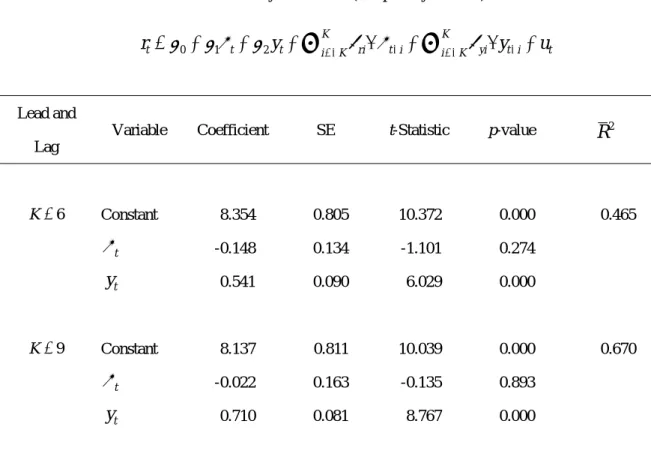
Since the existence of the cointegrating relation was supported, we estimated the Taylor rule. When we estimate the cointegrating vector, we cannot use the ordinary least squares (OLS) because we have a problem of endogeneity for regressors. In order to take into consideration this problem, we use the dynamic OLS (DOLS) method. We estimate the cointegating vector by adding

Δ π

_t and

Δ y

_t, and their leads and lags.

Table 2 shows the estimation results. As is evident from this table, the output coefficient is estimated to

5

be positive (0.541 for K = 6, and 0.710 for K = 9) and statistically significant in all cases at the 1% level.

On the other hand, the inflation rate coefficient is estimated to be negative (-0.148 for K = 6, and -0.022 for K = 9). However, the inflation coefficient is not statistically significant in any case.

4.2 Open-economy Taylor Rule

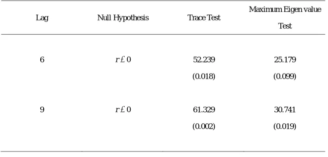
Next, we analyze India’s monetary policy reaction function by applying the Taylor rule augmented with exchange rate. Prior to estimation, we conducted Johansen-type cointegration tests for short-term interest rate, inflation rate, output gap, and real effective exchange rate. Table 3 shows the results of the cointegration tests. As is evident from this table, the null hypothesis of no cointegrating relation is rejected in three out of four cases at the 5% level. Thus, it is likely that there is a cointegrating relationship among interest rates, inflation rates, output gap, and exchange rate.

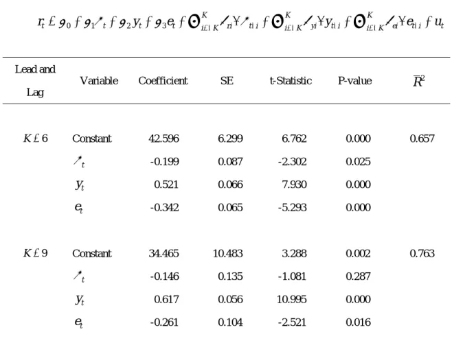
Since the existence of the cointegrating relation was supported, we estimated the extended Taylor rule using DOLS. We estimate the cointegrating vector in Equation (2) by adding

Δ π

_t,

Δ y

_t and

Δ e

_t, and their leads and lags. Table 4 shows the estimation results. As is evident from this table, the output coefficient is estimated to be positive (0.521 for K = 6, and 0.617 for K = 9) and statistically significant in all cases at the 1% level. The inflation rate coefficient is estimated to be -0.199 for K = 6 and -0.146 for K

= 9. These results are consistent with those obtained in Table 2. It is noted that the coefficient of the real effective exchange rate is estimated to be negative (-0.342 for K = 6, and -0.261 for K = 9) and is statistically significant in all cases at the 1% level.

5. Some Concluding Remarks

In 2008, the High Level Committee on Financial Sector Reforms submitted a report to the Indian government, recommending that “the RBI should formally have a single objective, to stay close to a low inflation number, or within a range, in the medium term, and move steadily to a single instrument, the short-term interest rate (repo and reverse repo) to achieve it” (GOI 2009 [5]). As epitomized by this proposal, given the recent volatile price movements, there are some arguments that the RBI has focused more on price stability in the conduct of monetary policy, and should further shift to inflation targeting.

This paper empirically analyzes India’s monetary policy reaction function by applying the simple Taylor rule and its open-economy version which employs dynamic OLS (DOLS). The analysis uses monthly data from the period of April 1998 to December 2007. When the simple Taylor rule was estimated for India, the

6

output gap coefficient was statistically significant, and its sign condition was found to be consistent with theoretical rationale; however, the same was not true of the inflation coefficient. When the open-economy Taylor rule was estimated, the coefficients of output gap and exchange rate had statistical significance with the expected signs, whereas the results of inflation remained the same as before.

These imply that the RBI could respond appropriately to internal supply-demand gaps and external competitiveness, but not to changes in price level. In other words, the short-term interest rate has not been the effective instrument in controlling the inflation rate. Therefore, based on empirical results, this paper concludes that it is inappropriate for the RBI to focus more on the inflation rate and adopt an Inflation- targeting type policy framework.

References  

Bhattacharyya, Indranil, and Rudra Sensarma. 2008. "How Effective are Monetary Policy Signals in India?." Journal of Policy Modeling 30, no.1: 169-183.

Chadha, Jagjit S., Lucio Sarno, and Giorgio Valente. 2004. "Monetary Policy Rules, Asset Prices, and Exchange Rates." IMF Staff Papers 51, no.3: 529-552.

Clarida, Richard, Jordi Gali, and Mark Gertler. 1998. "Monetary Policy Rule in Practice: Some International Evidence." NBER Working Paper, no.6254, November.

Clarida, Richard, Jordi Gali, and Mark Gertler. 2000. "Monetary Policy Rules and Macroeconomic Stability: Evidence and Some Theory." Quarterly Journal of Economics 115, no.1: 147-180.

Dickey, David A., and Wayne A. Fuller. 1979. "Distribution of the Estimators for Autoregressive Time Series with a Unit Root." Journal of the American Statistical Association 74, no.366: 427-431.

Fendel, Ralf M. and Michael R. Frenkel. 2006. "Five Years of Single European Monetary Policy in Practice: Is the ECB Rule-Based?." Contemporary Economic Policy 24, no.1: 106-115.

Government of India. 2009. A Hundred Small Steps: Report of the Committee on Financial Sector Reforms, New Delhi: GOI.

International Monetary Fund. 2008. International Financial Statistics. Washington, D.C.: IMF, April.

Jha, Raghbendra. 2008. "Inflation Targeting in India: Issues and Prospects." International Review of Applied Economics 22, no.2: 259-270.

Johansen, Søren. 1991. "Estimation and Hypothesis Testing of Cointegration Vectors in Gaussian Vector Autoregressive Models." Econometrica 59, no.6: 1551-1580.

7

McCallum, Bennett T. 1988. "Robustness Properties of a Rule for monetary Policy." Carnegie-Rochester Series on Public Policy 29, no.1: 173-203.

Mohan, Rakesh. 2008. "Monetary Policy Transmission in India." BIS Papers, no.35: 259-307.

Mohanty, M.S., and Marc Klau. 2004. "Monetary Policy Rules in Emerging Market Economies: Issues and Evidence." BIS Working Paper, no.149.

Peersman, Gert, and Frank Smets. 1999. "The Taylor Rule: A Useful Monetary Policy Benchmark for the Euro Area." International Finance 2, issue 1: 85-116.

Reserve Bank of India. 2006. Handbook of Monetary Statistics of India. Mumbai: RBI, March.

Reserve Bank of India. 2007. Macroeconomic and Monetary Developments First Quarter Review 2007-08.

Mumbai: RBI, July.

Reserve Bank of India. 2008. Macroeconomic and Monetary Developments in 2007-08. Mumbai: RBI, April.

Singh, Kanhaiya. 2006. "Inflation Targeting: International Experience and Prospects for India." Economic and Political Weekly 41, nos.27-28: 2958-2961.

Singh, Kanhaiya, and Kaliappa Kalirajan. 2007. "Monetary Transmission in Post-Reform India: An Evaluation." Journal of the Asia Pacific Economy 12, no.2: 158-187.

Taylor, John B. 1993. "Discretion versus Policy Rules in Practice." Carnegie-Rochester Conference Series on Public Policy 39, no.1: 195-214.

Taylor, John B. 2001. "The Role of the Exchange Rate in Monetary-Policy Rules." American Economic Review 91, no.2: 263-267.

Virmani, Vineet. 2004. "Operationalising Taylor-type Rules for the Indian Economy: Issues and Some Results (1992Q3-2001Q4)." IIMA Working Papers, no.2004-07-04.

8

Table 1 Cointegration Tests (

r

_t,

π

_t,

y

_t)

Lag Null Hypothesis Trace Test

Maximum Eigen value Test

6 r=0 32.620 22.117

(0.023) (0.036)

9 r=0 36.122 25.855

(0.008) (0.010)

Note:

r is the hypothesized number of cointegrating equations.

Numbers in parentheses are p-values.

9

Table 2 Dynamic OLS (Simple Taylor Rule)

t i t K

K

i yi

i t K

K

i ri

t t

t y y u

r =

^β

⁰ +

^β

¹

^π

+

^β

² +

∑

₌₋

^γ

Δ

^π

₋ +

∑

₌₋

^γ

Δ ₋ +

Lead and Lag

Variable Coefficient SE t-Statistic p-value

R

²

6

K = Constant 8.354 0.805 10.372 0.000 0.465

π

t -0.148 0.134 -1.101 0.274

y

t 0.541 0.090 6.029 0.000

9

K = Constant 8.137 0.811 10.039 0.000 0.670

π

t -0.022 0.163 -0.135 0.893

y

t 0.710 0.081 8.767 0.000

Note: SE is the Newey-West HAC Standard Error (lag truncation=5).

10

Table 3 Cointegration Tests (

r

_t,

π

_t,

y

_t,

e

_t)

Lag Null Hypothesis Trace Test

Maximum Eigen value Test

6 r=0 52.239 25.179

(0.018) (0.099)

9 r=0 61.329 30.741

(0.002) (0.019)

Note:

r is the hypothesized number of cointegrating equations.

Numbers in parentheses are p-values.

11

Table 4 Dynamic OLS (Open-economy Taylor Rule)

t K

K

i ei t i

i t K

K

i yi

i t K

K

i ri

t t t

t y e y e u

r =

β

₀ +

β

₁

π

+

β

₂ +

β

₃ +

∑

=−

γ

Δ

π

− +

∑

=−

γ

Δ − +

∑

=−

γ

Δ − +

Lead and Lag

Variable Coefficient SE t-Statistic P-value

R

²

6

K = Constant 42.596 6.299 6.762 0.000 0.657

π

t -0.199 0.087 -2.302 0.025

y

t 0.521 0.066 7.930 0.000

e

t -0.342 0.065 -5.293 0.000

9

K = Constant 34.465 10.483 3.288 0.002 0.763

π

t -0.146 0.135 -1.081 0.287

y

t 0.617 0.056 10.995 0.000

e

t -0.261 0.104 -2.521 0.016

Note: SE is the Newey-West HAC Standard Error (lag truncation=5).