A Weighted K
t,t-Free t-Factor Algorithm for Bipartite Graphs
Kenjiro Takazawa∗†
February, 2008
Abstract
For a simple bipartite graph and an integer t ≥ 2, we consider the problem of finding a minimum-weight t-factor under the restric- tion that it contains no complete bipartite graphKt,t as a subgraph.
Whent= 2, this problem amounts to the minimum-weight square-free 2-factor problem in a bipartite graph, which is NP-hard. We propose, however, a strongly polynomial algorithm for a certain case where the weight vector is vertex-induced on any subgraph isomorphic to Kt,t. The algorithm adapts the unweighted algorithms of Hartvigsen and Pap, and a primal-dual approach to the minimum-cost flow problem.
The algorithm is fully combinatorial, and thus provides a dual inte- grality theorem, which is tantamount to Makai’s theorem dealing with maximum-weight restrictedt-matchings.
1 Introduction
LetG= (V, E) be a simple undirected graph, that is,Ghas neither parallel edges nor self-loops. Throughout this paper, we assume that the given graphs are simple. For a vector b ∈ZV+, an edge set M ⊆ E is said to be a b-matchingif every vertex v ∈V is incident to at most b(v) edges in M, and a b-factor if every vertexv ∈V is incident to exactly b(v) edges inM. If b(v) = t for every v ∈ V, we simply refer to b-matchings/factors as t- matchings/factors. For instance, a 2-matching is a vertex-disjoint collection of cycles and paths, and a 2-factor is a vertex-disjoint collection of cycles that cover all vertices inV. If a b-factor exists in a graph, it is a maximum b-matching.
Let us denote a cycle of lengthkbyCk. For ab-matching/factorM with b(v)≤2 for eachv∈V, we say thatM isCk-freeifM contains no cycles of lengthk or less. The Ck-free 2-factor problem is to find a Ck-free 2-factor in a given graph. Note that the case where k ≤ 2 is exactly the classical simple 2-factor problem, which can be solved efficiently.
∗Department of Mathematical Informatics, Graduate School of Information Science and Technology, University of Tokyo, Tokyo 113-8656, Japan, and Research Insti- tute for Mathematical Sciences, Kyoto University, Kyoto 606-8502, Japan. E-mail:
†Supported by Grant-in-Aid for JSPS Fellows.
One important aspect of the Ck-free 2-factor problem is that it is a relaxation of the Hamilton cycle problem. From this point of view, it is easily seen that this problem is NP-hard when |V|/2 ≤ k ≤ |V| −1. Moreover, Papadimitriou showed that the problem is NP-hard when k ≥ 5 (see [1]).
On the other hand, for the case wherek= 3, an augmenting path algorithm is given by Hartvigsen [11]. TheC4-free 2-factor problem is left open.
The weighted Ck-free 2-factor problem is to find a Ck-free 2-factor that minimizes the total weight of its edges for a given weighted graph. The problem is NP-hard whenk≥5, which follows from the NP-hardness of the unweighted problem, and so is the case wherek= 4 [23]. The weightedC3- free 2-factor problem is unsettled. Polyhedral structures ofCk-free 2-factors are studied in Cunningham and Wang [3]. Related works also appear in [2, 14, 20].
We now focus on bipartite graphs. Note that it suffices to consider the cases wherek is even. While the C6-free 2-factor problem in bipartite graphs is NP-hard [10], C4-free 2-factors in bipartite graphs are tractable and studied actively. We remark that a C4-free 2-matching/factor in a bipartite graph, which is a 2-matching/factor that does not contain C4, is often referred to as a square-free 2-matching/factor. Since the complement of an (n−3)-connected bipartite graph is a square-free 2-matching, the theory of square-free 2-matching can be applied to the vertex-connectivity augmentation problem.
The first result on square-free 2-matchings was due to Hartvigsen [12], who proposed a characterization of graphs that admit square-free 2-factors and a combinatorial algorithm for finding one. This was followed by a min- max formula by Z. Kir´aly [15]. Then Hartivgsen [13], the journal version of [12], presented a full description of the algorithm and a constructive proof for the min-max formula.
As for the weighted Ck-free 2-factor problem in bipartite graphs, the NP-hardness when k ≥ 6 follows from that of the unweighted problem.
Moreover, Z. Kir´aly proved that the weighted square-free 2-factor problem is also NP-hard (see [6]).
An attractive generalization of the square-free 2-factor problem is the Kt,t-free t-factor problem, proposed by Frank [6]. In a bipartite graph, t- matching/factor is said to beKt,t-free if it contains no Kt,t as a subgraph.
Note that the case wheret= 2 is exactly the square-free 2-factor problem.
Using a general framework of Frank and Jord´an [7] on covering crossing bi-supermodular functions on pairs of sets, Frank [6] provided a min-max formula for Kt,t-free t-matchings, which extends Z. Kir´aly’s formula [15]
for the spacial case of t = 2. Through this approach, one can compute the size of the maximum Kt,t-free t-matching in polynomial time by the ellipsoid method or a combinatorial method by Fleiner [5]. Moreover, one can find a maximumKt,t-freet-matching combinatorially by applying V´egh and Bencz´ur’s algorithm for covering pairs of sets [22]. A direct approach to this problem was done by Pap [17, 18, 19]. He gave a combinatorial proof for Frank’s min-max formula, which implies a polynomial-time algorithm.
We remark that applying Pap’s algorithm to the case whent= 2 results in
an algorithm different from Hartvigsen’s algorithm.
The weightedKt,t-freet-factor problem in bipartite graphs has also been considered. As mentioned, this problem is NP-hard when t= 2. However, Makai [16] showed a linear programming description of maximum weight Kt,t-free t-matchings and proved its dual integrality for a certain class of weight vectors called vertex-induced. For a weight vector w ∈ RE and a subgraphH ofG,wis said to be vertex-induced onH if there exists a func- tionπH :V(H)→Rsuch thatw(uv) =πH(u)+πH(v) for everyuv∈E(H).
Here,V(H) andE(H) denote the vertex set and edge set ofH, respectively, and uv denotes an edge connecting u, v ∈ V(H). The class considered by Makai [16] is thatw is vertex-induced on any subgraph isomorphic to Kt,t. Applying the ellipsoid method to Makai’s description, one obtains a poly- nomial algorithm for this class of weighted bipartite graphs, which could be made strongly polynomial by Frank and Tardos’ method [8].
This paper presents a combinatorial primal-dual algorithm to find a minimum-weightKt,t-freet-factor in a weighted bipartite graph whose weight vector is vertex-induced on any subgraph isomorphic to Kt,t. The primal part of the algorithm is a variant of Hartvigsen’s and Pap’s algorithms, while the dual part is based on the framework of a primal-dual approach to the minimum-cost flow problem [4, 21]. The algorithm is fully combinatorial, so the output of the algorithm is integer if the weight vector is integer. Thus, the algorithm implies a theorem on dual integrality of an LP-formulation for the problem, which is tantamount to Makai’s one [16]. The complexity of the algorithm is O(tn2D), wherenis the number of vertices andDis the time to execute a shortest path algorithm with nonnegative length. Incor- porating Fredman and Tarjan’s implementation of Dijkstra’s algorithm [9], we get a strongly polynomial complexity O(tn2m+tn3logn), where m is the number of edges.
This paper is organized as follows. Section 2 describes a maximum- cardinality square-free 2-matching algorithm, and Section 3 extends it to a minimum-weight square-free 2-factor algorithm. Section 4 provides a fur- ther extension of the algorithm to the weighted Kt,t-free t-factor problem.
Finally, Section 5 discusses the relation between minimum-weight Kt,t-free t-factors and maximum-weightKt,t-free t-matchings.
Before closing this section, let us prepare some notations and definitions used in the following sections. LetG= (V, E) be an undirected graph with vertex setV and edge setE. An edge connectingu, v∈V is denoted byuv.
For a vertexv∈V,δv⊆Edenotes the set of edges incident tov. ForZ ⊆V, the subgraph induced byZ is denoted byG[Z] = (Z, E[Z]), that is,E[Z] = {uv|u, v∈Z,uv∈E}. For a subgraphHofG,V(H) andE(H) denote the vertex set and edge set ofH, respectively, i.e.,H = (V(H), E(H)). A cycle is a subgraph ({v1, . . . , vk},{e1, . . . , ek}) wherevi 6=vj ifi6=j, ei =vivi+1
fori= 1, . . . , k−1 andek =vkv1. A cycle consisting ofk edges is denoted byCk.
When we denote a graph byG= (U, V;E), we mean thatGis bipartite, that is, the vertex set and edge set ofGareU∪V andE, respectively, and E[U] andE[V] are empty. For subgraphHofG,U(H) (resp.V(H)) denotes
the set of vertices in U (resp. V) that belong to H. A complete bipartite graph Ks,t is a simple bipartite graph (U, V;E) with |U|=s, |V|=t and E={uv|u∈U,v∈V}. Recall thatK2,2 is isomorphic toC4, and is often called a square. For a subgraph H of G, a component in H isomorphic to K2,2 is called asquare-componentand the number of square-components in H is denoted by c(H). For a bipartite graph G, letSt denote the family of all its subgraphs isomorphic to Kt,t. We often abbreviate S2 asS.
For a directed graph G= (V, A) with vertex set V and edge set A, we denote an edgeefromutovbyuv, as far as it causes no confusion whethere is directed or undirected. Fore=uv∈A, the initial and terminal vertex of eare denoted by∂+e and∂−e, respectively, that is, ∂+e=u and ∂−e=v.
A path is a subgraph ({v1, . . . , vk},{e1, . . . , ek−1}) where vi 6= vj if i 6= j and ei =vivi+1 fori= 1, . . . , k−1.
For two sets F1, F2 ⊆E, the symmetric difference (F1\F2)∪(F2\F1) is denoted by F14F2. For a vector x ∈ RE and F ⊆ E, define x(F) =
∑
e∈F x(e).
2 A Maximum Square-Free 2-Matching Algorithm
This section describes an algorithm to find a maximum square-free 2-matching in bipartite graphs. The algorithm is based on algorithms of Hartvigsen [12, 13] and Pap [17, 18, 19], but different from both. Our algorithm uses the shortest augmenting path, whereas Pap’s one does not involve the length of augmenting paths. Using the shortest path yields some simplicity, espe- cially in the shrinking procedure, which makes the algorithm suitable for a weighted extension.
Let G= (U, V;E) be a bipartite graph and M ⊆E be a square-free 2- matching inG. First, construct an auxiliary directed graphGM = (U, V;A) in the following manner. Define the directed edge setA by
A={uv|u∈U,v∈V,uv ∈E\M} ∪ {vu|v∈V,u∈U,uv∈M}. Where it causes no confusion, we identify the undirected edgeuv inGand the directed edge uv (or vu) inGM. We also define two distinguished sub- setsU◦⊆U and V◦ ⊆V by
U◦ ={u|u∈U,|δu∩M|<2}, V◦ ={v|v∈V,|δv∩M|<2}. Then, find a shortest path P from U◦ to V◦ and consider the edge setM0=M4E(P). Observe thatM0 is a 2-matching with|M0|=|M|+ 1.
Hence, ifM0 is square-free, then M0 is a larger square-free 2-matching. We refer to the procedure to obtain M0 as an augmentation.
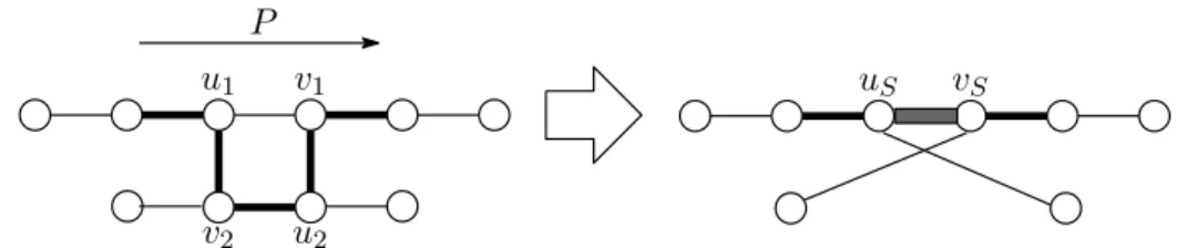
What if, however, M0 contains squares? Suppose M4E(P) contains a squareS. SinceP is the shortestU◦-V◦path, we have that|M∩E(S)|= 3, a detailed discussion of which will appear in Proposition 2.1. DenoteU(S) = {u1, u2},V(S) ={v1, v2}and {u1v1}=E(P)∩E(S) (see Figure 1). Then, what we do is to “shrink”S. Identifyu1 and u2 to obtain a new vertexuS, and v1 and v2 to obtain a new vertex vS. Then, delete all edges in E(S)
u1 v1
v2 u2
uS vS P
Figure 1: Shrinking of a square (bold line :M-edge).
and connect uS and vS by an M-edge. If an edge in E \E(S) had been incident to u1 or u2 (resp. v1 or v2), the edge is incident to uS (resp. vS) in the resulting graph. We allow parallel edges to appear in this procedure.
If an edge had belonged toM, it also belongs toM in the new graph, and otherwise it does not. We denote the resulting graph by ˜G= ( ˜U ,V˜; ˜E) and refer to the newM-edge uSvS as ashrunk square. Note that it follows from
|M ∩E(S)|= 3 that the number of M-edges in the parallel edges incident touS (or vS) is at most one, so M remains simple whereas ˜Gmay not. In addition, the new M is a 2-matching in ˜G and may contain a square that includes shrunk squares.
If more than one square appears in M4E(P), we shrink the square which is “closest” toU◦. That is, we shrink the square whose non-M-edge appears the first inP. We refer to the procedure to obtain a new graph and 2-matching asShrink(M, P).
Then, we recursively execute the above procedures. Here, we have to take care that theU◦-V◦ path does not contain shrunk squares. In order to achieve this, we search aU◦-V◦ path in a subgraph ˜G0M of ˜GM obtained by deleting all the shrunk squares. Then, setb∈ {1,2}U˜∪V˜ by
b(v) = {
1 (v is an end vertex of a shrunk square deleted from ˜GM),
2 (otherwise), (1)
and modify the definition ofU◦ andV◦ by
U◦={u|u∈U ,˜ |δu∩M|< b(u)}, V◦ ={v|v∈V ,˜ |δv∩M|< b(v)}. (2) This means that what we deal with is a square-free b-matching M in ˜G0M. Thus, one would see that the shrunk squares get neither incident to each other nor nested.
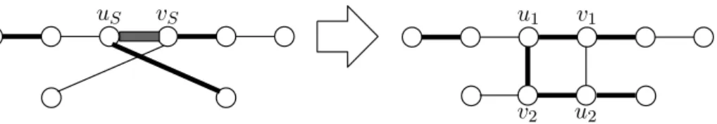
After an augmentation, we expand every shrunk squares to obtain the original bipartite graphG. Let uSvS be a shrunk square that is obtained by shrinking S with U(S) = {u1, u2} and V(S) = {v1, v2}. Now, replace the vertices uS, vS and edge uSvS by K2,2 induced by U(S)∪V(S). An edge incident to uS or vS is connected to a vertex in U(S)∪V(S) to which the edge had been incident before shrinking S. Next, determine M-edges. An M-edge before expanding S also belongs to M. Then, pick up three edges inE(S) to be in M so that M forms a 2-matching. Figure 2 illustrates an example of expanding a shrunk square. By expanding every shrunk square, we obtain the original bipartite graphGand a new square-free 2-matchingM of one larger size.
uS vS
v2 u2
u1 v1
Figure 2: Expanding of a square (bold line :M-edge).
The procedures are summarized below.
Algorithm Maximum Square-Free 2-Matching Step 0: SetM =∅ and ˜G=G.
Step 1: If|M|= 2 min{|U|,|V|}, then halt. (M is a square-free 2-factor.) Step 2: Construct an auxiliary directed graph ˜G0M. In ˜G0M, definebby (1)
and search for a shortest path fromU◦ to each vertex. LetR⊆U˜∪V˜ be the set of the reachable vertices from U◦. If V◦ ∩R = ∅, then expand each shrunk square and halt. (M is a maximum square-free 2-matching.)
Step 3: LetP be the shortest path from U◦ toV◦. If M4E(P˜ ) contains a square in ˜G0M, then execute Shrink(M, P) and go to Step 2.
Step 4: ReplaceM by M4E(P˜ ) and expand every shrunk square. Then, go to Step 1.
Here, we show that ifM4E(P˜ ) contains a squareSthen|M∩E(S)˜ |= 3.
Proposition 2.1. Let S be a square in G˜0M that appears in M4E(P).˜ Then, it holds that |M ∩E(S)|˜ = 3.
Proof. Since ˜E(S)⊆ M4E(P˜ ), the edges in ˜E(S) can be partitioned into two parts, ˜EM =M∩E(S) and ˜˜ EP = ˜E(P)∩E(S). We prove that˜ |E˜P|= 1.
As M is square-free in ˜G0M, we have that |E˜P| ≥ 1. As P visits each vertex at most once and the edges ofM and E\M lie alternately inP, we have that|E˜P| ≤2. Hence, it suffices to show that |E˜P| 6= 2.
Denote U(S) = {u1, u2} and V(S) = {v1, v2}. To the contrary we as- sume, without loss of generality, that ˜EP ={u1v1, u2v2} and u1v1 appears earlier than u2v2 in P. Let us denote the subpath of P which is from the initial vertex ofP tov1byP1, and which is fromu2 to the terminal vertex of P byP2. Here, connectingP1,u2v1 and P2, we obtain another U◦-V◦ path, which is shorter thanP. This contradicts thatP is the shortestU◦-V◦ path in ˜G0M.
Now, what is left is to prove that M is maximum when the algorithm halts in Step 2. The following is a min-max formula for square-free b- matchings.
Theorem 2.2 (Z. Kir´aly [15]). Let G= (U, V;E) be a bipartite graph and b∈ {0,1,2}U∪V. Then, the size of the maximum square-free b-matching in Gis equal to
Z⊆U∪Vmin {b(U ∪V \Z) +|E[Z]| −c(G[Z])}.
Let us view the weak duality and equality conditions for the formula.
ForG= (U, V;E) and b∈ {0,1,2}U∪V, define a functionfG,b : 2U∪V → R by
fG,b(Z) =b(U ∪V \Z) +|E[Z]| −c(G[Z]).
LetM be a square-freeb-matching andZ ⊆U∪V. ForZ, partitionM into three sets M1, M2, M3, where
M1 =M ∩E[Z], M2=M∩E[(U ∪V)\Z], M3=M \(M1∪M2).
Then, it follows that
|M1| ≤ |E[Z]| −c(G[Z]), 2|M2|+|M3| ≤b(U ∪V \Z). (3) Hence, it holds that
|M| ≤ |M1|+ 2|M2|+|M3| ≤fG,b(Z). (4) By (3), we have the following conditions for (4) to hold with equality.
Condition (a). In G[Z], every edge except for one edge in each square- component belongs toM.
Condition (b). M2 =∅.
Condition (c). ∀v∈(U∪V)\Z,|M3∪δv|=b(v).
In what follows, we abbreviatefG,basfG, sincebis always defined by (1).
We prove that there existsZ ⊆U∪V such that|M|=fG(Z), which yields a verification of our algorithms and an alternative proof for Theorem 2.2. The argument below is an adaptation of the combinatorial proof for Theorem 2.2 of Pap [17, 18, 19] to our algorithm.
The following is a key observation to our verification.
Proposition 2.3. LetS0 ={S|S ∈ S, S is shrunk into uSvS in G˜ }. Then, foruS of S ∈ S0,G˜0M has a path fromU◦ touS consisting of edges that was in a shortest path used in shrinking a square S0 ∈ S0 and closer to U◦ than uS0.
Proof. The proof is by induction on the number of shrinkings. The state- ment is obvious immediately after shrinkingS.
Now, suppose P is a path fromU◦ to uS that satisfies the condition in the statement and consider subsequent shrinkings. A shrinking that does not delete any edge in ˜E(P) does not matter. If a shrinking deletes an edgee∈E(P˜ ), then it holds thate∈M. For, ife6∈M, a squareSe appears wheneturns to be anM-edge by Proposition 2.1, which contradicts thate
uS vS
vS uS e
uS00 vS00
Figure 3: Reachability of uS (bold line :M-edge).
had been in a shortest path used in shrinkingS0 ∈ S0 and closer to U◦ than uS0. Lete∈M∩E(P) be deleted in a subsequent shrinking (an example is˜ shown in Fig. 3). Here,∂−e∈U˜ is shrunk intouS00, which is reachable from U◦. On the other hand,uS is reachable fromuS00 by tracing the subpath of P that had connected ∂−e anduS. Therefore, the statement is maintained in shrinkingS00.
Suppose no U◦-V◦ path is found in Step 2 and denote the current graph ˜G0M by G0 = (U0, V0;E0). Recall that we deleted all the shrunk squares from ˜GM to obtain ˜G0M. Let R ⊆ U0 ∪V0 be the set of vertices reachable from U◦ in ˜G0M, and define Z0 = (U0 ∩R)∪(V0 \R). For Z0, partitionM into three setsM1, M2, M3, where
M1=M∩E[Z0], M2 =M∩E[(U0∪V0)\Z0], M3 =M\(M1∪M2).
Then, by the definition ofZ0, it holds that
|M1|=|E[Z0]|, |M2|= 0, M3 =b(U0∪V0\Z0), c(G[Z0]) = 0, and hence|M|=fG0(Z0). By (4), it follows thatM is the maximum square- freeb-matching in G0 and Z0 minimizesfG0.
Next, consider to expand a shrunk square. LetZ0∗⊆U0∪V0be a minimal minimizer offG0. That is,f(Z0∗)< f(Z0) holds for allZ0(Z0∗. LetuSvS be a shrunk square inG0and denote the bipartite graph obtained by expanding uSvS byG1 = (U1, V1;E1). Consider whether uS, vS ∈Z0∗ or not.
By Proposition 2.3, G0 has a path P from U◦ to uS which consists of edges that was in a shortest path used in shrinking a square and closer to U◦ than the square. Denote the initial vertex of P by u0. Since u0 ∈ U◦, Condition (c) implies that u0 ∈ Z0∗. Moreover, carefully looking at Conditions (a) and (b), we have thatU0(P)⊆Z0∗andV0(P)⊆(U0∪V0)\Z0∗, which implies that uS ∈Z0∗.
Therefore, we have two cases: vS ∈Z0∗ or not.
Case 1 (vS∈Z0∗). Define Z1 ⊆U1∪V1 by Z1 = (Z0∗\ {uS, vS})∪U(S)∪ V(S). Then, it is easily seen that
b((U1∪V1)\Z1) =b((U0∪V0)\Z0∗), E1[Z1] =E0[Z0∗] + 4.
Moreover, it holds that c(G1[Z1]) = c(G0[Z0∗]) + 1. For, by Condi- tion (a) no edge in E[Z0∗] is incident to uS, and if an edge in E0[Z0∗] is incident tovS then Z0∗\ {vS} also satisfies Conditions (a)–(c) and minimizes fG0, which contradicts the minimality of Z0∗. Hence, the subgraph induced byU1(S)∪V1(S) is a square-component inG1[Z1], which implies thatc(G1[Z1]) =c(G0[Z0∗]) + 1.
Therefore, we have that fG1(Z1) = fG0(Z0∗) + 3. Since the size of M increases by three in expanding a shrunk square, it holds that
|M| = fG1(Z1). Thus, it follows from (4) that M is a maximum square-free b-matching inG1 and Z1 is a minimizer of fG1.
Case 2 (vS6∈Z0∗). DefineZ1 ⊆U1∪V1 byZ1 = (Z0∗\ {uS})∪U(S). Then, it holds that
b((U1∪V1)\Z1) =b((U0∪V0)\Z0∗) + 3, E1[Z1] =E0[Z0∗], c(G1[Z1]) =c(G0[Z0∗]),
and hence|M|=fG1(Z1). Then, by (4), we have thatMis a maximum square-free b-matching inG1 and Z1 is a minimizer of fG1.
Applying the above argument repeatedly, we obtain a square-free 2- matchingM in the original graphGandZ ⊆U∪V such that|M|=fG(Z).
3 A Weighted Square-Free 2-Factor Algorithm
This section deals with the weighted square-free 2-factor problem. Let (G, w) be a weighted bipartite graph withG= (U, V;E) andw∈RE+. Throughout this section, we assume that |U| = |V|. We also assume that w is vertex- induced on any square. That is, we assume that, for any square S with U(S) ={u1, u2} and V(S) ={v1, v2}, there exists a potential function πS : U(S)∪V(S)→Rsuch thatw(uivj) =πS(ui) +πS(vj) for anyi, j∈ {1,2}. In other words, it holds that w(u1v1) +w(u2v2) =w(u1v2) +w(u2v1). We propose an algorithm to find a square-free 2-factorM that minimizesw(M) if exists, or otherwise determine that no square-free 2-factor exists in G.
The algorithm, based on the primal-dual framework of the minimum-cost flow algorithm [4, 21], extends Algorithm Maximum Square-Free 2- Matching.
Let x ∈ RE. The following is a linear programming relaxation of an integer program for the minimum-weight square-free 2-factor problem:
(P) minimize wx
subject to x(δv) = 2 (∀v∈U ∪V), x(E(S))≤3 (∀S∈ S), 0≤x(e)≤1 (∀e∈E).
One would see that the incidence vector of a square-free 2-factor is a feasible solution for (P). In what follows, we often identify an edge set M and its incidence vectorx.
Consider the dual problem of (P). Let p∈RU∪V,q ∈RE and r ∈RS. The dual problem is given by
(D) maximize 2(p(U)−p(V))−q(E)−3r(S) subject to p(u)−p(v)−q(e)− ∑
S:e∈E(S)
r(S)≤w(e) (∀e=uv ∈E), q, r≥0.
The complementary slackness conditions of (P) and (D) are x(e)>0⇒p(u)−p(v)−q(e)− ∑
S:e∈E(S)
r(S) =w(e), (6)
q(e)>0⇒x(e) = 1, (7)
r(S)>0⇒x(E(S)) = 3. (8)
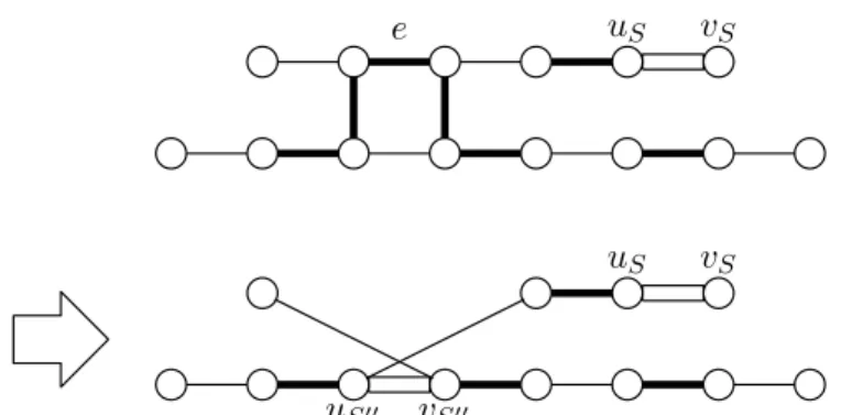
In what follows, we present an algorithm to find feasible solutions for (P) and (D) which satisfy (6)–(8) by extending Algorithm Maximum Square-Free 2-Matching. Roughly speaking, we maintain a square- free 2-matchingM, construct an auxiliary directed graph ˜GM, search for a U◦-V◦ path P in its subgraph ˜G0M, and then augment M by substituting M4E(P˜ ) for M or shrink a square. In these procedures, we also take dual solutions into account. In particular, a significant difference from Algo- rithm Maximum Square-Free 2-Matchingis that we do not expand a shrunk square uSvS after an augmentation if r(S)> 0, and such a shrunk square is used in the subsequent searching for aU◦-V◦ path.
Now, let us consider the details. Let ˜GM = ( ˜U ,V˜;A) be an auxiliary directed graph, which may have resulted from repeated shrinking and ex- panding of squares. Recall that theM-edges (including all shrunk squares) are oriented in the direction from ˜V to ˜U, and other edges in the opposite direction. For ˜GM, a length functionl:A→R is defined by
l(e) =
w(e)−p(u) +p(v) (e6∈M and corresponds to uv∈E),
−w(e) +p(u)−p(v) (e∈M and corresponds to uv∈E), r(S) (eis a shrunk squareuSvS).
Remark that p is defined on U∪V, the vertex set of the original bipartite graphG, while lis defined on A, the edge set of ˜GM.
In the auxiliary graph ˜GM, we establish the following optimality crite- rion.
Theorem 3.1. Let M be a 2-factor in G˜M such that each square in M contains shrunk squares, and let p ∈ RU∪V and r ∈ RS. If the following (9)–(11) hold, then we can expand M to obtain a minimum-weight square- free 2-factor in (G, w) and determine q so that (p, q, r) forms an optimal solution for (D):
r ≥0 and r(S)>0 only if S is shrunk; (9)
∀e∈A, l(e)≥0; (10)
∀shrunk square uSvS, ∀e=uv ∈E(S), p(u)−p(v)−r(S) =w(e). (11)
Proof. We prove the theorem by showing how to construct feasible solutions for (P) and (D) that satisfy (6)–(8).
Let e=uv ∈ E be an edge not shrunk in ˜GM. If e6∈M, then by (10) we have thatl(e) = w(e)−p(u) +p(v)≥0. Now, set q(e) = 0 to have (6) and (7) hold ine. If e∈M, then l(e) = −w(e) +p(u)−p(v) ≥0 by (10).
Setq(e) =l(e), which gets (6) and (7) to hold in e.
Let e = uv ∈ E belong to E(S) of a shrunk square uSvS in ˜GM. For such e, set q(e) = 0. Then, by (11), we have that (6) and (7) hold in e regardless whetherx(e) = 0 orx(e) = 1 after expandingS.
Now we have determinedq(e) on everye∈E. From the above construc- tion, one would appreciate the feasibility of (p, q, r) for (D). Moreover, by expanding all shrunk squares in ˜GM, we obtain a square-free 2-factor inG, a feasible solution for (P). For this pair of solutions for (P) and (D), it follows from (9) that (8) holds. Therefore, (6)–(8) hold for this pair of solutions for (P) and (D).
Now, let us describe the minimum-weight square-free 2-factor algorithm.
The algorithm keeps a square-free 2-matchingM and a dual solution (p, r) that satisfy (9)–(11), and increases |M|until it attains the maximum.
Algorithm Minimum-Weight Square-Free 2-Factor Step 0: SetM =∅,p= 0, r= 0 and ˜G=G.
Step 1: If|M|= 2|U˜|, then expand every shrunk square and halt. (M is a minimum-weight square-free 2-factor.)
Step 2: Construct an auxiliary directed graph ˜GM = ( ˜U ,V˜;A) and delete shrunk squares that are created after the latest augmentation to obtain a new graph ˜G0M. Then, in ˜G0M, definebby (1) and search for a shortest path with respect to (w.r.t.)l fromU◦ to each vertex. LetR⊆U˜∪V˜ be the set of the reachable vertices fromU◦ and defined: ˜U∪V˜ →R by
d(v) =
{distance fromU◦ tov w.r.t.l (v∈R), max{d(v)|v∈R} (otherwise).
IfV◦∩R =∅, then halt. (No square-free 2-factor exists.)
Step 3: LetP be the shortest path (w.r.t l) from U◦ toV◦. If more than one shortest path exists, select a path with the minimum number of edges. If P contains a shrunk square, apply Dual-Update (described below), expand every shrunk square inP, and then go to Step 2.
Step 4: IfM4E(P˜ ) contains a square without shrunk squares, applyDual- Update, execute Dual-Shrink(M, P) (described below), and then go to Step 2.
Step 5: Apply Dual-Update, replace M by M4E(P), and expand every˜ shrunk squareS withr(S) = 0. Then, go to Step 1.
We remark that a shrunk square uSvS with r(S) > 0 is not expanded in Step 5, and belongs to ˜G0M after the augmentation.
In the procedure Dual-Update, we change the dual solution as follows:
p(v) :=p(v)−d(v) (v∈U ∪V), r(S) :=
{r(S)−d(uS) +d(vS) (S is shrunk),
r(S) (otherwise),
whered(v) for a vertexv∈(U∪V)\( ˜U∪V˜) that is shrunk intovS ∈U˜∪V˜ is defined byd(vS).
The procedure Dual-Shrink(M, P) is twofold: update of p in two ver- tices; and Shrink(M, P). We have that M4E(P˜ ) contains squares in ˜G0M. For such a square S, it holds that |M ∩E(S)˜ | = 3, which is proven later (Proposition 3.2). LetS be the nearest one from U◦ among the squares in M4E(P˜ ), and denote ˜U(S) ={u1, u2} and ˜V(S) ={v1, v2}. Without loss of generality, we assume u1v1 ∈E(P)˜ \M. Then, update the values p(u2) and p(v2) by
p(u2) :=p(u2)−l(u2v1), p(v2) :=p(v2) +l(u1v2), and call Shrink(M, P).
Now, let us confirm the validity of the algorithm. Note that (9)–(11) hold at the beginning of the algorithm. We prove that the conditions are maintained throughout the algorithm.
Proposition 3.2. Throughout the algorithm, the following(i) and(ii)hold:
(i) l(e)≥0 for each edge ein G˜0M,
(ii) if a square S without shrunk squares appears in M4E˜(P), it holds that|M∩E(S)˜ |= 3.
Proof. We prove that (ii) holds under the assumption of (i), and (i) is main- tained when (ii) holds. Then, since (i) holds at the beginning of the algo- rithm, (i) and (ii) inductively hold throughout the algorithm.
LetS be a square without shrunk squares such that ˜E(S)⊆M4E(P˜ ).
Denote ˜U(S) ={u1, u2}, ˜V(S) ={v1, v2}, and ˜EP = ˜E(P)∩E(S). By the˜ argument in the proof for Proposition 2.1, it suffices to show that |E˜P| 6= 2 in order to prove (ii).
Assume to the contrary that ˜EP ={u1v1, u2v2}andu1v1appears earlier than u2v2 in P. Then, it holds that ∑
e∈E(S)˜ l(e) = 0 since w is vertex- induced on S. Hence, it follows from (i) that l(e) = 0 for all e ∈ E(S).˜ Now, as is described in the proof for Proposition 2.1, we have anotherU◦- V◦ pathP0, which is obtained by takingv1u2 as a shortcut forP. It follows from (i) andl(v1u2) = 0 thatP0, which has fewer edges thanP, is no longer thanP w.r.t. l. This contradicts the choice of P.
Next, we prove that (i) is maintained under the assumption of (ii). Con- siderDual-Update. Pick up a directed edge e∈A. By the definition of d, it holds that d(∂−e)≤d(∂+e) +l(e). If e=uv is in the direction from ˜U to
V˜, the shift ofl(e) inDual-Update is−(−d(u))−d(v) =d(∂+e)−d(∂−e)≥
−l(e). If e=vu is not shrunk and in the direction of ˜V to ˜U, i.e., e∈M, then the shift of l(e) is −d(u)−(−d(v)) =−d(∂−e) +d(∂+e)≥ −l(e). Fi- nally, ife= vSuS is a shrunk square, the shift of l(e) is −d(uS) +d(vS) =
−d(∂−e) +d(∂+e) ≥ −l(e). Therefore, in any case we have that l(e) ≥ 0 after Dual-Update. Moreover, for a shortest U◦-V◦ path P, the above in- equalities hold with equality for each e ∈ E(P) and hence˜ l(e) = 0 after Dual-Update. Thus, in an augmentation using P, in which l(e) changes to
−l(e) fore∈E(P˜ ), (i) is maintained.
ConsiderDual-Shrink(M, P). Since (ii) holds, the procedureDual-Shrink(M, P) is valid. InDual-Shrink(M, P),lchanges only on the edges inδu2∪δv2. One would easily see thatl(u1v2) andl(u2v1) become zero by the update ofp(u2) and p(v2). As we have applied Dual-Update just before Dual-Shrink(M, P), we have l(u1v1) = 0. Moreover, since w is vertex-induced on S, it holds that l(u2v2)−l(u1v1) = l(u1v2) +l(u2v1), which implies that l(u2v2) also becomes zero. Meanwhile, for an edgee∈(δu2∪δv2)\E(S), we have that e6∈M. Hence, the shift of l(e) is equal tol(u2v1) for e∈δu2 and equal to l(u1v2) fore∈δv2. Therefore,l(e)≥0 is kept for every edge inδu2∪δv2 in Dual-Shrink(M, P).
The above argument induces the following corollaries.
Corollary 3.3. After Dual-Update, l(e) = 0 for every edgee∈E˜(P).
Corollary 3.4. When we shrink a square S, l(e) = 0 for everye∈E(S).˜ It follows from Corollary 3.4 that (11) holds for S when we shrink S, which is the purpose of the update ofp(u2) andp(v2) inDual-Shrink(M, P).
Proposition 3.5. Let uSvS be a shrunk square created after the latest aug- mentation. Then, d(uS) = 0 until the next augmentation.
Proof. It follows from Proposition 2.3 thatuSis reachable fromU◦in ˜G0M by traversing edges that had been in a shortestU◦-V◦ path. By Corollary 3.3, such an edge e has its length l(e) = 0 in Dual-Update executed when e ∈ E(P˜ ), andl(e) remains to be zero until the next augmentation.
Proposition 3.6. Throughout the algorithm, (9)–(11) hold.
Proof. Condition (9). Since we change r(S) only if S is shrunk and ex- panduSvSonly ifr(S) = 0, it holds thatr(S) = 0 for every non-shrunk square S. Moreover, we have seen in the proof for Proposition 3.2 that r(S) = l(uSvS) ≥ 0 for every shrunk square uSvS in ˜G0M. As for a shrunk square not in ˜G0M, in other words created after the latest shrunk, d(uS) = 0 by Proposition 3.5, which implies r(S) ≥ 0 after aDual-Update. In Dual-Shrink(M, P),r(S) is not changed since Dual- Shrink(M, P) is executed for a square containing no shrunk square.
Condition (10). Already proved.
Condition (11). By Corollary 3.4, (11) holds whenS is shrunk. Consider the shift ofp(u)−p(v)−r(S) in subsequentDual-Updatefore=uv ∈ E(S). The variables are changed as follows:
p(u) :=p(u)−d(uS), p(v) :=p(v)−d(vS), r(S) :=r(S)−d(uS) +d(vS).
Then, p(u)−p(v)−r(S) does not change in Dual-Update. In Dual- Shrink(M, P), the variables concerned are not changed.
By Theorem 3.1 and Proposition 3.6, if the algorithm halts in Step 1, then we have a minimum-weight square-free 2-factorM and a dual optimal solution. If the algorithm halts in Step 2, G has no square-free 2-factor.
This is shown by a similar argument to that in Section 2.
Let us discuss the complexity of the algorithm. Recall that|U∪V|=n and |E|=m. The following is an easy observation, but plays a key role in analyzing the complexity.
Proposition 3.7. A shrunk square created in Step 4 is not expanded until the next augmentation.
Proof. We search a U◦-V◦ path P in ˜G0M, which does not contain shrunk squares created after the latest augmentation, and a shrunk square expanded by the next augmentation is contained inP.
The bottleneck part of the algorithm lies in Step 2, determining the distance from U◦ to every vertex. It follows from Proposition 3.2 that this can be computed by a shortest path algorithm with nonnegative length. By Proposition 3.7, we apply a shortest path algorithm O(n) times between augmentations. Since augmentations happen at most n times throughout the algorithm, the total complexity of the algorithm is O(n2D), where D is the time to execute a shortest path algorithm with nonnegative length.
Among a number of implementations of such an algorithm, incorporating Fredman and Tarjan’s version of Dijkstra’s algorithm [9], we get a strongly polynomial complexity O(n2m+n3logn).
Theorem 3.8. Algorithm Minimum-Weight Square-Free2-Factor runs inO(n2m+n3logn) time.
We should remark here thatAlgorithm Minimum-Weight Square- Free 2-Factor is fully combinatorial, that is, it consists of only addition, subtraction, and comparison. Thus, the algorithm leads to the following integrality theorem.
Theorem 3.9. Let(G, w)be a weighted bipartite graph such thatGadmits a square-free2-factor andw∈RE+is integer and vertex-induced on any square.
Then, the linear program (P) has an integral optimal solution. Moreover, the dual problem (D)also has an integral optimal solution(p, q, r) such that the elements in{S |S ∈ S, r(S)>0} are pairwise disjoint.
4 Extension to K
t,t-Free t-Factors
We can naturally extend Algorithm Minimum-Weight Square-Free 2-Factorto the minimum-weightKt,t-freet-factor problem. Let (G, w) be a weighted bipartite graph with G= (U, V;E) andw ∈RE+. Assume that
|U|=|V|and w is vertex-induced on anyKt,t inG.
Let x∈RE,p∈RU∪V,q ∈RE and r ∈RSt. The following is a linear programming relaxation of an integer program for the minimum-weightKt,t- freet-factor problem:
(Pt) minimize wx
subject to x(δv) =t (∀v∈U∪V), x(E(S))≤t2−1 (∀S ∈ St), 0≤x(e)≤1 (∀e∈E).
The dual problem of (Pt) is
(Dt) maximize t(p(U)−p(V))−q(E)−(t2−1)r(St) subject to p(u)−p(v)−q(e)− ∑
S:e∈E(S)
r(S)≤w(e) (∀e=uv∈E), q, r≥0.
We describe an algorithm for the minimum-weightKt,t-freet-factor prob- lem by mentioning the differences from Algorithm Minimum-Weight Square-Free 2-Factor. First, let us remark Dual-Shrink(M, P). As an extension of Proposition 3.2, we have the following.
Proposition 4.1. Throughout the algorithm, the following(i) and(ii)hold:
(i) l(e)≥0 for each edge ein G˜0M,
(ii) if aKt,t, denoted byS, appears inM4E(P), then˜ |M∩E(S)˜ |=t2−1.
LetSbe aKt,tinM4E(P) closest from˜ U◦. Denote ˜U(S) ={u1, . . . , ut} and ˜V(S) = {v1, . . . , vt}, and suppose u1v1 6∈ M. We update the dual valuable as follows:
p(ui) :=p(ui)−l(uiv1), p(vi) :=p(vi) +l(u1vi) (i= 2, . . . , t).
Sincew is vertex-induced onS, we have l(e) = 0 for everye∈E(S) by this˜ update.
Then, we shrink S in the following manner. Identify the vertices ˜U(S) to obtain a new vertexuS, and ˜V(S) to obtain a new vertexvS. Delete all edges in ˜E(S) and connectuS andvS by an M-edge. If an edge in ˜E\E(S)˜ had been incident to ˜U(S) (resp. ˜V(S)), the edge is incident to uS (resp.
vS) in the resulting graph. If an edge had belonged to M, it also belongs to M in the new graph, and otherwise it does not. We refer to the new M-edge uSvS as a shrunk Kt,t.
Next, in an auxiliary directed graph ˜G0M, the vectorb is defined by
b(v) =
1 (v is an end vertex of a shrunkKt,t deleted from ˜GM), 2 (v is an end vertex of a shrunkKt,t in ˜G0M),
t (otherwise).
(12)
Then,U◦ and V◦ are determined by (2) according to (12).
Now, we are ready to present a full description of an algorithm to find a minimum-weightKt,t-free t-factor.
Algorithm Minimum-Weight Kt,t-Free t-Factor Step 0: SetM =∅,p= 0, r= 0 and ˜G=G.
Step 1: Letkbe the number of shrunkKt,t in ˜G. If|M|= 2k+t(|U˜| −k), then expand every shrunk Kt,t and halt. (M is a minimum-weight Kt,t-free t-factor.)
Step 2: Construct an auxiliary directed graph ˜GM = ( ˜U ,V˜;A). In ˜GM, delete every shrunk Kt,t that is created after the latest augmentation to obtain a new graph ˜G0M. Then, in ˜G0M, definebby (12) and search for a shortest path w.r.t.l fromU◦ to each vertex. Let R⊆U˜∪V˜ be the set of the reachable vertices fromU◦ and define d: ˜U ∪V˜ →R+
by
d(v) = {
distance fromU◦ tov w.r.t.l (v∈R), max{d(v)|v∈R} (otherwise).
IfV◦∩R =∅, then halt. (No Kt,t-free t-factor exists.)
Step 3: LetP be the shortest path (w.r.t l) from U◦ toV◦. If more than one shortest path exists, select a path with the minimum number of edges. If P contains a shrunkKt,t, apply Dual-Update, expand every shrunkKt,t inP, and then go to Step 2.
Step 4: If M4E(P) contains a˜ Kt,t without a shrunk Kt,t, apply Dual- Update, execute Dual-Shrink(M, P), and go to Step 2.
Step 5: Apply Dual-Update, replace M by M4E(P˜ ) and expand every shrunkS∈ St withr(S) = 0. Then, go to Step 1.
Let us discuss the complexity. Recall thatn=|U∪V|,m=|E|andDis the time for a shortest paths algorithm with nonnegative length. In Step 4, we check whetherM4E(P˜ ) contains aKt,t, which takes O(m) time, smaller than the complexity of a shortest path algorithm. Hence, it takes O(nD) time between augmentations. Since augmentations happen at most tn/2 times, the total complexity is O(tn2D), which gets to O(tn2m+tn3logn) by employing D= O(m+nlogn) [9].
Theorem 4.2. Algorithm Minimum-WeightKt,t-Freet-Factorruns in O(tn2m+tn3logn) time.