An Inventory Model with Dependent Intervals of Demand

(1)

J. Operations Research Soc. of Japan Vo!. 18, No.1 & 2, July 1975

AN INVENTORY MODEL WITH DEPENDENT INTERVALS

OF DEMAND

MICHIKO SORIMACHI Tokyo Institute of Technology (Received June 19, 1973; Revised January 17, 1974)

Abstract

The inventory problem for continuous time is studied in which the demand process is composed of two different processes, one is a compound Poisson process and the other is a generalized semi-Markov chain or a process whose intervals of occurrence are constant.

We assume that holding and shortage costs are convex. And a set-up charge for ordering are considered.

The form and bounds of an optimal policy are determined and some numerical results in the special case are added.

Finally, we consider some combined policy at the view point of practical use and compare with a simple (s, S) policy.

1. Introduction

It is usually assumed that demand are independently and identically distributed in different periods, and in the con-tinuous case, assumed that intervals of demand are subject to an exponential distribution. The case of arbitrary interval distribution has been ana1yzed in [1] and [2], where independent intervals of demand are assumed.

We consider, for example, the situation where a part of demand is required by fixed customers and other part, by a

(2)

Inventory with Dependent Intervals of Demand 65

floating purchasing power. In such Cl case, intervals of demand

are no longer independent.

We treat such a case and develop the continuous inventory model with the following two types of demand (type 1 and type 2) •

Those are superposed of a compound Poisson process and the other process: type 1 has a constant interval of occurrence with an independent and identical distribution of demand size, and type 2 is a generalized semi Markov chain. Type 2 is an extension of type 1.

Section 2 gives the structure of the model.

Section 3 presents a proof of the optimality of an (s(t), Set)) policy where t denotes a parameter defined in §3.

In section 4, we discuss about Cl special demand process

of type 2 that is a superposition of two compound Poisson processes.

Section 5 gives upper and lower bounds of the optimal critical numbers for N truncated decision periods.

In section 6, numerical examples are given, observing the effect of parameter t.

Since optimal policy (s(t), Set») are very complicated both in calculation and practical use, section 7 presents a relatively simple policy which is a combined policy of (s, S) policy and not always optimal, but in some cases, is better than simple (s, S) policy.

(3)

2. Notations and the Model

We formulate the model more precisely. Following notations are used.

x:

y: q,2

(O :

inventory before ordering inventory after ordering

the probability distribution function of demand size of compound Poisson process, one component of superposition of two processes.

q,l{~): that of the other component of superposition T: deterministic delivery 1ag

g{y): an expected holding and shortage cost function

A:

parameter of interval of compound Poisson process Following assumptions are made.

1. Decisions concerning whether to order stock replace-ments and how much to order may be immediately after a demand has arisen.

2. Delivery of an order is assumed to require a fixed time,

T.

3. No restriction is placed on the size or number of orders that may be outstanding at any time.

4. There is a fixed cost of ordering, K, which is incurred when the order is made.

5. A holding and shortage penalty cost is charged against inventory level after

T

time later after ordering.

g{y) is a non negative convex function in y with g{y) ~ 00 as

Iyl

~ 00

(4)

Inventory with Dependent Intervals of Demand

6. Complete backlogging is postulated.

7. Future costs are discounted by a discount rate e-a per unit time.

8. Since no disposal is permitted, y > x at the same point of time.

9. Infinite planning horizon is assumed.

Since interest cost is included in holding cost, the un-avoidable outlay of the purchasing price per item need not be considered.

The decision objective is to minimize the expected value of present and discounted future avoidable cost.

3. Inventory Equations and Form of an Optimal Policy

67

First, we shall consider type 1. If we call compound Poisson process C type and the other process ,,,i th constant interval (T) D type, type 1 is a superposition of C type and D type.

Let fD(y) denote the expected value of discounted avoidable cost at a time immediately after a demand of D type, having present stock level y, if an optimal policy is followed.

Also, fc(t, y), for 0 < t < T, denotes the expected value of discounted avoidable cost at a time immediately after a demand of C type which occurs at time T-t after D type occurred, having present stock level y, if an optimal policy is followed.

Now, we define fc(T, y) :: fD(y) expediently, and moreover, abbreviate index c, then f(t, y) :: fc(t, y) for 0 < t < T with-out confusion.

(5)

Here, we will introduce the functional equation that f(t, x) satisfies. Consider the system immediately after a demand of type D has occurred. We pay attention to time when first C type demand occurs after the origin, occurrence time of

D

type. Let i t be (t, t+dt). When kT < T < (k+l)T for k=2, 3,

• • • I we classify the following six cases • (1) For 0 < t < T,

only C type demand occurs during an interval (T, T+t) (2) For

T < t < T-T, nothing occurs during an interval (T, t) and only

C type demand occurs during an interval (t, T+t) (3) For

T-T < t < kT, nothing occurs during an interval (T, t), and

only C type during (t, T), D type occurs at T and only C type occurs during (T, T+t) (4) For kT < t < T, nothing occurs during (T, t), only C type during (t, T), D type at T, only C type during (T, T+t) (5) For T < t < T+T, noting occurs during

(T, T),

D

type at T, nothing during (T, t), only C type during (t, T+T) (6) For T+T < t, nothing occurs during (T, T), D type at T, nothing during (T, T+T).

The cost of storage or shortage during an interval of length t if t < T and length T if t ~ T, but placed T units of time later, is considered. We denote the discounted cost of storage and shortage expected with the demand size distribution during a time interval (t₁, t₂) with stock level y, by L(y, tl t₂) .

Based on the above classification, we obtain the following functional equation. We have1)

(6)

Inventory with Dependent Intervals of Demand

-f(T,X) inf(Koo(y-x) +! Ae T -At {L(Y,T,T+t) + e

=-=--

-at ! 00 f(T-t,y-~)d~2(~)}dt

y~x 0 ~=O t-T -At -at 00 +!_ Ae {L(Y,T,T+t)+e ! f(T-t,y-~)d~2(~)}dt T ~O kT + ! T -At

=-=--

-at

+ ! _AOe {L(y,T,T+t) + e ! f(T-t,y-~)d~2(~)}dt

kT ~=O

T+T -At ~ -aT 00

+! Aoe {L(y,T,T+T) + e ! f(t,y-~)d~l(~)}dt

T ~=O

00

-At ~ -aT

+! Aoe {L(y,T,T+T) + e ! f(T,y-~)d~l (~)}dt)

T+T ~=O

00

69

Calculating each L(y, t l t 2} for six intervals where demand occurrences are given above, and integrating by t and summing up, we denote i t by LT(y} °

Then, f(T, x} satisfies the functional equation

(3ol) f(T,x) ~nf{Koo (y-x)+~(y)+! . T ! ),oe -(A+a)t f(T-t,y-~)d~2 (~)dt

(3 ° 2)

y~x t=O ~=O

And for T > 2T,

+

e-(A+a)~?!oo f(T,y-~)d~l (~)}

~=O

+ (e-(A+a)T_e-(A+a) (T+T»{

~

L. (Ai)j+l (j+l) ~ - G1,j+l (y)+G1,o(y)}),

(7)

70 where 2 )

(3.3) G, ,(y)

1,J

When T < 2T, the same functional eg. (3.1) holds, but for l < T < i T ' ,

(3.4) LT(y) = A.Ui[(e 1 -IA+a)T -e -(A+a)T) L (A;,j+l (' 1) I ·G

o ' l(y)

+a j=l J + . ,J+

1 -AT -CtT -aT -(Ha)T 00 j+l j+l (Ha)R,-j- 2 6_T)R,

+ - e (e -e ) 9 (y) -e L A GO' +1 (y) L

-'-'-'-='-;R,:-;:---!..~'-"--a j=l ,J R,=O

1 1

For k+l < T < k' k 1, 2, . . .

_1_1 L (AT)j+l(G ( ) . ( -<A+a)T_ -(A+a) (k+l)T) A+a j=l (j+l)! k,j+l y e e G ( ) ( -(Ha) (k+l)T -(A+a) (T+T) + k+l,j+l y • e -e - (A+a) (k+l)T j+l . e L (kT_T)J-r+l

eT)

j+l r=O x

-A(k+l)T ( ) 1( a -(A+a)T -A(k+l)T-aT + _A_ e-(A+a) (k+l)T)

x e Gk,o Y +;:; >:+;;e -e A+a

x G (y) + ~_ ( -a(k+l) T-A (T+T) _ -(Ha) (T+T»G ( )

kl o. e e k+l,O y

2):

~(i)

is the i-fold convolution of

~

with itself.

*

denotes convolution mark.

(8)

Inventory with Dependent Intervals of Demand 71

Especially for

T

0,

(3.6) L ( ) _{T Y} ₌ _Ha1 {l _- _e-(Ha)T} ( ) _g _y

In the same way, f(t, x) for 0 < t < T, satisfies the

functional equation

(3.7) flt,x) - inf{K"6(y-x) + Lt(y) + f t f A"e - (A+a) T f(t-T,y-~)dTd~2(~) ~-o

y~x T-O

-(A+a)t 00

+ e f f(T,y-~)d~l(~)}' ~-O

where Lt(y) denotes the discounted expected cost of storage or shortage cost during an interval between the origin t and next first occurrence of demand, but placed ~ units of time later.

(3.8)

For T

=

0,

Lt(y) = ___ 1 ___ (1 _ e-(A+a)t)g(y) A+a

From the above functional eqs. (3.1) and (3.7), we will derive the form of an optimal policy. So we introduce the following lemma which can be deriven by slitely rewritting Theorem 2.1 in Kalymon [3].

Lemma. Let

E

be any subspace of N dimensional Euclid space. For arbitrary U ~

E

and any real number x, the follow-ing function f(u, x) is defined, where Lu(Y) is a convex func-tion of y and p(vlu) is a funcfunc-tion satisfying dP(vlu) > 0 and

f dP (v

I

u) ~ l . E

(1) f(u,x)

y~x

inf{K·6 (y-x) + Lu(Y) + f f dP(vlu) f(v,y-Od~ (O}

Vf!

E

~=O v

Then, f(u,x) has an optimal policy of the (s(u), S(u» form. The above lemma shows the following.

Theorem 3.1. For demand process of type 1, there exists an optimal policy of the (s(t), S(t» form (0 < t < T).

(9)

Michiko Sorimachi

Proof. It suffices to show that eqs. (3.1), (3.7) are included in the special case of eq. (1). If we put P(ult) for 0 < t < T as follows

P(TI t)

for 0 < T < t,

then eqs. (3.1) and (3.7) are rewritten

(3.9) f(t,x) = inf{Koo(y-x) + Lt(y) + J

J

dP(ult)f(u,y-t)d~ (O},

y~,x ufE ~=O u

,..;

where E (0, t) U T and ~u(~)

=

~2(~) for u ~ T and otherwise

~u(~)

=

~l(~)' Lt(y) is convex function of y from assumptions in section 2, so the results is deriven from the above lemma.

In the same way, we will give the functional equation of an optimal cost function of type 2. In type 2, state i of a generalized semi Markov chain implies that the distribution of the size of demand is ~i' We call Ai type for state i. The joint distribution function of state j after v or less v time later given that the state is i, is denoted by F(v, jli).

fA. (y): expected value of discounted avoidable cost at

l

a time immediately after a demand of Ai type, conditional on inventory y and an optimal policy.

fc(t, i, y): expected value of discounted avoidable cost at a time immediately after a demand of C type which occurs at time t after Ai type occurred, conditional on inventory y and an optimal policy.

(10)

Inventory with Dependent Intervals of Demand

Then, fA. (y) and fc(t, i, y) satisfy the functional

~

equations

(3.10)

y~x

inf {Ko(y-x) + LA. (y) + E 1

~ j v=O x 1 fe(t,i,y-~)d~2(~) ~=O -At -ay

I

+

E l l

Ae e dvF(V, j i)dtl fA (y-~)d~.(~)} j v=O t=v ~=O j J

inf {K·o (y-x) + LA. (y) + 1

y~x ~ t=O

where dF(vli) _ EdF(v, jli), F(tli) =1 dF(vli),

j ~~

F(B, jli) =1 e-SvdF(V, jli)

v=o

(3.11) fe(t,i,x)= inf {K·o(y-x) + L(t,i) (Y)

Y~x

where d~(i, t, v, j) denotes the joint distribution of residual time v and next state j at time t after state i, in semi Markov chain. dvK(i,t,v) - ~dvK(i,t,v,j), K(i,t,T)

J

(11)

00

- f dVK ( i , t , v),

K (

i , t, j , 8) _ f e - 8v dvK ( i , t , v , j )

v=~ v=o

And LAi(y) and L(t,i) (y) denote analogous meanings of Lt (y) in type 1.

-In the case of T 0,

1 -v

A+a{l-F(A+ali) }g(y)

L(t,i)(y) A!a{l-1((i,t,A+a) }g(y)

Thus, we obtain the following

Theorem 3.2 For demand process of type 2, there exists an optimal policy of the (5 (u), S (u)) form, where U E

E,

E= {Ai' (t,i), i=1,2, ... , 0 < t < oo}

Proof In the same manner of Theorem 3.1, we put

i, j = 1,2, . . .

dP((t,i)ls

i) = Ae-(A+a)t .P(tli) for 0 < t < 00, i=1,2, •.. P (S j I (t, i)) =

'K' (

i , t , j , A +a) for 0 < t < 00, i=l, 2, •..

dP( (t+T, i) I (t,i))

for 0 < t < 00, i=1,2, .••

Then, eqs. (3.10) and (3.11) are reduced to the same type as eq. (1) of lemma and the results are obtained.

(12)

4. Special case of type 2: in the case of a compound Poisson demand process

In the demand process of type 2, we take specially a compound Poisson process of parameter A2 as a semi Markov demand process, so superposition of two process is also a compound Poisson process. In this case, we will try two different methods of analysis and show that those results are consistent.

For a compound Poisson process with a parameter A

=

Al + A2 and the probability distribution function of denand size, f(Al <1>2 + A

2<1>l)' the optimal cost function satisfies the following functional equation.

-For simplicity, we assume T = O.

(4.1. ) f (x) inf {K·O(y-x) + A+a .g(y) 1

y~x

vlhile, according to the argument in section 3, eqs. (3.10)

and (3.11), for a superposition of t:wo compound Poisson processes with parameter Al and A2 and the probability dis-tribution of demand size, <1>1 and <1>2' respectively, we show that the optimal cost function satisfies the same functional equation as (4.1).

Since in eqs. (3.10) and (3.11)

A!a· g (y),

'K

(t, /3)

(13)

76

1

L (t, i) (y) = A+cl·g (y) ,

the optimal cost functions fA, (x) and fc(t,x) satisfy the

~ functional eqs. (4.2) fA, (x) J. (4.3) fc (t,x) 1 inf {K·6(y-x) + A+a g(y) y~x

+ f f

t=O ~=O

' f { " ) 1 () f f -(A+a)'r_f ( ~)

J.n K·u(y-x + A+a· g y + e c t+'r, y-s

y~x T =0 ~=O

Now, we take fc(t,x)

=

h(x) independent of t, eqs. (4.2) and (4.3) coinside with each other, and fAi (x)

=

fp(t,x)

=

h(x). Moreover, this satisfies eq. (4.1). Since eqs. (4.1), (4.2),

(4.3) have unique solution (See [3]), we have f(x) = h(x).

5. Bounds on s(u), S(u)

We define fn(n > 1) by the following equation.

I

n-l

inf {K.6(y-x) + Lu(Y) + f f dP(v u)f (v,y-~)

(14)

where u,

E,

Lu(Y}' p(vlu} are defined in eq. (I)

Remark: We call fn n truncated decision period case. And under appropriate conditions, fn(u, x} converges f(u, x}

in eq. (I) as n + 00 monotonically and uniformly in any

finite interval. (See [3])

We denote critical numbers in eq. (S.l) as sn(u} and Sn(u}. Then, specially for demand process of type 1 and type 2 bounds on sn(u}, Sn(u} are given in the following theorem.

Theorem 5.1 For demand processes of type 1 and type 2,

(S.l)

where ~(u), s(u}, ~(u), S(u} are defined as following.

(S.2)

(S.3)

(S.4)

where

(S.S)

min Lu(Y} = Lu(~(U}} y

Let ~(u) be the smallest number such that

Define s(u} as the smallest number such that

D(u} 1 {A + a·e-(A+a}u}, 0 < u < T, for a demand A+a

process of type 1,

(15)

78 (5.6)

and

(5.7)

D(u)

D(u) f d K(j,t,v) A!a{A + a.e-(A+a)v}

o

v

for u = (t,j), in a demand process of type 2.

Define S(u) as the smallest number greater than §..(u)

for which (5.8)

Proof: The method of proof is followed as same line as Veinott & Wagner [7], B. A. Kalymon [3]. So we will show only the outline.

(1) The Proof of §..(u) ~ Sn(u) for all u, n.

Let Y_n be an optimal policy with sn(u), Sn(u) structure with Sn(u) ~ §..(u) for some n, u.

Define the policy Yn' by

r~U)

for _xn < sn (u) , u _n u

Yn

,

for xn > sn(u) un

=

u

Yn for un

t-

u

and for i

=

n-l, n-2,

.

,

1, y .

,

max{x_i ' , y. }, where x.

,

1 1 1

represent the inventory in period i when following Yi'.

(16)

Also, either Yi'

=

Yi' in which case LUi(Yi') = Li(Yi) or Y· < y.' ~ S(u) and theorefore, by convexity of Lu(Y) and

1 1 - - '

the definition of ~(u)

Then for xn

Since fn(u,xIY_n)

=

fn(u,xIY

n') for all othe~ un' and for un u with xn ~ _{sn(u), we have shown that Yn}

is

not an

optimal policy, which

is

contradiction. (2) The proof of ~(u) ~ sn(u)

Suppose for an optimal policy Y , s (u) _n _n < _-s(u) for some n, u. By (1), S(u) ~ Sn(u).

such that

Let Y I be an alternative policy

n

rn(U)

for xn < sn (u) , S(u) for sn(u) < _xn

Yn

,

t:

for xn > ~(u) , for un

"

u and for i = n-l, n-2, ... , 1, Yi'

Then, as in similar argument 3): E denotes expectation mark.

un

=

u

< ~(u), u _n

=

u

un u

nax{x i ', Yi}·

(17)

80

for un

=

u, with sn(u) < xn diction.

x < ~(u). This is a

contra-(3) The proof of sn(u) ~ s(u).

Let Y_n be an optimal policy with s(u) < sn(u), Define Yn' by

r

Sn(u) for xn < s(u) , U n U

Y

,

for s (u) ,

)"n

xn > U U n n for _un~ U \ Yn

\-.-and for i = n-1, n-2, ••• , 1, Yn' = _{Yn '}

For un

=

U and s(u) < xn

=

x < sn(u), at first consider type 1, then

fn(u,x/Y ) - fn(u,x/Y ')

=

K + L (S (u»

n n u n

Here, the notation of E is a expectation mark with respect to demand size. Remark that x_n_₁ (also x_n_₁') is a different random variable according to the occurence time of demand, t < u or t ~ u. But in any way, 8(Y_n_1 - x_n_{_1 ) 8(Yn_1}

(18)

Inventory with Dependent Intervals of Demand

Then, we obtain

fn(u,xly) - fn(u,xly ') ~ (l-D(u»'K + L (S(u» - L (s(u» ~ 0,

n n u - u

where D(u) for type 1.

In an analogous manner, for un and for type 2,

u and

s

(u) < xn

and

We put

and

fn(u,xly) - fn(u,xly ')

=

K + L {S (u» - L (x)

n n u n u + E {E J d F(v,klj) k 0 v v -At -at f Ae e dt[K·8(y I - x )

o

n- n-l 00 l O O - A t -ay - K'8(Y n_1 - xn_l')] + E {E _{k 0}f d F(v,k j) _v f _vAe e dt[K·8{y _n-I for u

fn(u,xly) - fn{u,xly ')

=

K + L (S (u» - Lu(X)

n n u n v -At -at + E f dvK(j,t,v) f Ae e dt[K.8{Y n_1 - Xn_l)

o

0 for u (t, j)

D(u) f d F (v

I

j) I {A+ a'e-{A+a)v} for u A.

o

v A+a ] D(u) f d K(j ,t,v) I

o

v Ma -'{A+a)v 0.+ (l'e } for u (t, j) 81

(19)

Michiko Sorimachi

Then, the same reason for type 1, we obtain

So, Yn' is also an optimal policy. Repeating the procedure for every u for which s(u) < sn(u), we arrive at an optimal policy for which sn(u) < s(u) for all u.

(4) The proof of Sn(u) ~ S(u).

Let Y_n be an optimal policy with Sn(u) > S(u) and define Yn' by

y ,

n

and for i

=

n-l, n-2, . . . , 1, Yi'

=

Yi. Then, in the same manner as (3), for xn

u

x < sn(u) and

> L (S(u» - L (S(u)) - K·D(u) ~ 0

= u u

-Thus Yn' is also an optimal policy. Repeating the pro-cedure for every u for which S(U) < Sn(u), we arrive at an optimal policy for which Sn(u) ~ s(u) for all u, as required.

(20)

6. Some Examples

We calculate optimal policies for a special case of type 1 whose component processes have both deterministic demand size, for compound Poisson process demand size is 1 and for other process i t is M. We consider all variables discrete, then consider that intervals of Poisson process

k-l

follo\ved geometric distribution, p(X k) = p.q , k = 1,2,

For

T

critical numbers are as follows.

(6.1) < sn(t) __ < - [l-S.KJ r·S where S denotes discount rate.

y > 0

bounds of optimal

y < 0

We calculate in n truncated decision case, and apply i t for infinite time horizon. (in our examples, convergences are attained in n ~ 20).

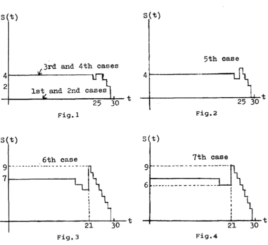
We take the cases where T 30, M 30, h 1.0, q 0.1 6 0.9 and r k 1st case 9.0 2 2nd case 99.0 2 3rd case 9.0 8 4th case 99.0 8 5th case 999.0 8 6th case 999.0 30 7th (~t:. _99.0 ₃₂ 83

(21)

84

From (6.1), sn (t) only Sn(t).

o

for all cases and we calculate

Fig. 1 ~ 4 illustrates how S(t) varies with t. Since time t denotes that C type demand occurs at time T-t after D type occurred, we conjecture that when t is near T(=30), S(t) gets small, because next occurrence of D type is far and C type demand is low.

Thus, we would estimate that S(t) is first constant in some interval and next increases up some levels and then decreases linearly to zero.

s(t)

5th

case

3rd and 4th cases

4

2

1st and 2nd

t

Fig.l Fig.2

s(t)

s

t)

6th case

7th case

9 --- - ---

9 ---.----7~---_t

6

---~---~21~-~3~0-t

₂₁

₃₀

_t Fig.3 Fig.4

(22)

7. A Further Consideration

We consider same demand process as type 1 in §6. An optimal policy (s(t), S(t}} is so complicated both in calcu-lation and in practical use that, observing the results of examples in §6 we present a combination of the simple strate-gies that is not always optimal but will be better than the

simple (s, S) policy in some cases.

In [4], Popp discussed the simple strategies as above, but, from his assumption of independent intervals between de-mands, any combined policy can not be better than simple (s, S) policy and his results are erroneous.

Add following assumptions to those in §2.

1. T = 0

2. The holding costs are given per unit of time and unit of quantity by h.

3. A discount can be neglected. 4. No delay is allowed.

5. M is relatively large and an inventory level can not exceed M.

6. A stocking level Q is discrete variable.

The criterion of optimization are minimal costs per unit of time. From above Assumption 1 and 4, optimal s(t} = O.

Now, we define three strategies, Policy 1, Policy 2 and Policy 3.

Policy 1: a simple (s, S) policy

(23)

Policy 2: a directly ordered policy, that is a policy without stock on hand

Policy 3: a combined policy where decision of a simple (s,8) policy is followed for some interval length t1 (t

1 > 0) and after the time t ₁, directly ordered policy is followed.

Let C

1(Q) and C3(Q, t1) be respectively the costs per unit of time and C₁(Q, t) and C

3(Q, t1, t) the costs over time interval (O,t), following policy 1 and 3 with stock on hand Q. From the above assumption 5, Q < M. Then, a time when a demand with constant intervals occurs, is always an ordering point and a renewal point under this inventory process.

As well known results of renewal theory,

C1 (Q,T) Q K 00 *kQ

Cl (Q)

=

T

=

2h + 1'(1 + L G (T)) for M > Q, k=l

(7.1)

where G(t) denotes the exponential distribution with parameter A and G*l(t) the 1 th convolution of G(t), that is 1-Er1ang distribution.

As for policy 3, we use following notations.

Xi: interval of ordering when Policy 1 is followed. They have an independent and identical Q-Er1ang (G*Q) distribution.

N(t): the number of ordering until time t. Then, for x ~ t1 > 0,

P(N(t1 ) = k, x ~ X₁+ . . . +Xk ~ x+dx) t

f _{19 *(k-1)Q(y) .g*Q(x-y)dydx}

(24)

where g*Q(x)

dG*Q(x) dx using the above,

(7.2) C 3(Q,t1,T) = 1: f C3(Q,t1,TIN(t1)=k, x1+ ••• +Xk=x)dP(N(t1) k, k=l 0 where 00 T 1: f {K·(k+A(T-x»+ h.~}dP(N(tl)=k,Xl+ ••• +Xk=X) k=l x=tl 00 00 + 1: f {K.k + h·2!} dP(N(t1)=k,X1+ ••• +xk=x) k=l x=T 2 hnT hnT *" hnT = K + = + (KAT-=)·G "(T) + (K-KAT+=)·M ( t ) 2 2 2 Q 1 !::2. T *Q + (2 -KA)f x·g (x)dx, x=t 1 1: G *kQ (t), mQ (t) k=l CXMQ(t)

=

dt

Of course, from (7.1) and (7.2),

C

3 (Q, T, T) = Cl (Q, T) Now, we calculate an optimal t l .

(25)

(704)

(7.5)

x m (t )oG*Q(T-t) - (hQ_KA)ot oM ( t ) + (h2Q-KA)otIoGf*Q(tl)

Q I I 2 I Q I

+ (KA - hQ) oTo (M (T) - GQ(T»

2 Q

Now, for policy 2,

c

= ~ + KA

2 T

As in [41, the comparison of inventory policies uses the policies with optimized decision variables, and the sign

> is used for a preference, then

(7.6) P2 < PI for kA > 2h

From (7.4), if kA >

~M

and AT < 1 for example,

hM

Then, if kA

>:1

and AT < 1 P3 ,> PI > P2

(26)

Acknowledgement

The author wishes to express her deepest appreciation to Prof. H. Morimura for his helpful suggestions and advices.

References

[1] Arrow, K. J, Karlin, S and Scarf, H, Studies in the Mathematical Theory of Inventory and Production, Stanford, California, Stanford University Press (1958) Chapters 16 and 17.

[2] Beckffiann, M, "An Inventory Model for Arbitrary Interval and Quantity Distributions of Demands", !Vlanagement Sci. 8-1 ('61)

[3] Kalymon, Basil A, "Stochastic Prices in a Single-Item Inventory Purchasing Model", Operations Research 19-6

( '71)

[4] Popp,

vI,

"Simple and Combined Inventory Policies, Pro-duction to stock or to order?", Management Sci. 11-9

( , 65)

[5] Scarf, H., "The Optimality of (5, s) Policies in the Dynamic Inventory Problem", Chap 13 in Math. Methods in the Social Sciences, K.J. Arrow, S. Karlin, and S. Suppes (eds.), Stanford University Press (1960)

89

[6] Veinott, A. F. Jr., "Optimal Policy in a Dynamic Single Product, Nonstationary Inventory Model with Several Demand Classes", Operations Research 13-5 ('65)

[7] Veinott, A. F. Jr. and Wagner H. M., "Computing Optimal (s,S) Inventory Policies", Management Sci. 11-5 ('65)