TWO EFFICIENT ALGORITHMS FOR THE GENERALIZED MAXIMUM BALANCED FLOW PROBLEM

Journal of the Operations Research Society of Japan

Vol. 45, No. 2, June 2002

TWO EFFICIENT ALGORITHMS FOR THE GENERALIZED MAXIMUM BALANCED FLOW PROBLEM

Akira Nakayama Chien Fei Su Fukushima University Tokuritsu Co. Ltd. (Received October 23, 2000; Final December 25, 2001)

Abstract Minoux considered the manmum balanced /low problem, i.e. the problem of finding a maximum flow in a two-terminal network

Af

= (V, A) with source s and sink t satisfying the constraint that any arc-flow of

Af

is bounded by a fixed proportion of the total flow value from s t o t , where V is vertex set and A is arc set. Several efficient algorithms, so far, have been proposed for this problem. As a natural generalization of this problem we focus on the problem of maximizing the total flow value of a generalized flow in a network

Af

= (V, A) with gains ?(a) > 0 (a E A) satisfying any arc-flow of

Af

is bounded by a fixed proportion of the total flow value from s t o t, where ?(a) f (a) units arrive a t the vertex w for each arc-flow f (a) ( a '= (v, w ) E A) entering vertex v in a generalized flow in

At.

We call it the generalized maximum

balanced flow problem and if ?(a) = 1 for any a E A then it is a maximum balanced flow problem. The authors believe that no algorithms have been shown for this generalized version. Our main results are t o propose two polynomial algorithms for solving the generalized maximum balanced flow problem. The first algorithm runs in O(mM(n, m, B') log B ) time, where B is the maximum absolute value among integral values used by an instance of the problem, and M(n, m, B f ) denotes the complexity of solving a generalized maximum flow problem in a network with n vertices, and m arcs, and a rational instance expressed with integers between 1 and B'. In the second algorithm we combine a parameterized technique of Megiddo with one of algorithms for the generalized maximum flow problem, and show that it runs in O({M(n, ~ X , B ' ) } ~ ) time.

1. Introduction

Minoux [7] considered the maximum balanced flow problem, i.e. the problem of finding

a maximum flow in a two-terminal network

N

= (V, A) with source s and sink t satisfying the constraint that the value of any arc-flow of Af is bounded by a fixed proportion of the total flow value from s to t , where V is vertex set and A is arc set. Such a constraint is described in terms of a balancing rate function a : A -+

R+

-

{O}

with a ( a ) :< 1 (a A), where R+ is the set of nonnegative reals. The maximum balanced flow problem is motivated by Minoux's research of reliability analysis of communication networks. If a flow from source s t o sink

t

is balanced, then it is guaranteed that the value of the blocked arc-flow is at most the fixed proportion of the total flow value from s to t. So far, several algorithms ([l]

,

[7], 181, [9], (1 21) have been proposed for the maximum balanced flow problem. They contain a network simplex method without cycling, and a parameterized maximum flow algorithm, and a binary search method and so on. The latter two run in polynomial- time. For the problem of finding an integral maximum balanced flow, Zimmermann [12]

showed this problem is W-hard, where Cui [l] gave an efficient algorithm in the case when the balancing rate function is constant. On the other hand, Ichimori et al [5] considered the weighted minimax flow problem and proposed a couple of polynomial algorithms for this

problem, and Fujishige et al. [3] have pointed out the equivalence of the maximum balanced

flow problem and the weighted minimax flow problem.

Generalized Balanced Flow Algorithms 1 63

By the way, we can study some directions for generalizing the maximum balanced flow problem. There is a problem of discussing the kernel or null space {x : Qx = 01 of any real matrix Q in place of the circulation space which is the kernel of the vertex-arc incidence matrix of the underlying graph with a new arc (t, s) attached. Zimmermann [12] treated another direction of generalization of the problem, i.e. the maximum balanced submodular flow problen over totally ordered commutative groups. In this paper we focus on generalized maximum balanced flow problem, i.e. the problem of maximizing the total flow value of a generalized flow in a network

N

= (V,

A )

with gains ~ ( a )

>

0 (a 6 A) satisfying the value of any arc-flow of

N

is bounded by a fixed proportion of the total flow value from s to t,

where ~ ( a ) f (a) units arrive a t the vertex

w

for each arc-flow f (a) (a = (v, w) E A) entering

vertex u in a generalized flow in

N.

The generalized maximum balanced flow problem with

gains ?(a) = 1 (a G A) is equivalent to the maximum balanced flow problem.

The objective of the present paper is to propose two efficient algorithms. The authors believe that no algorithms, so far, have been shown for the generalized maximum balanced flow problem. The complexity of the first algorithm is O(nM(n, m, B') log

B) time, where

B is the maximum absolute value among integral values used by an instance of the gener-

alized maximum balanced flow problem, and M(n, m,

B'}

denotes the complexity of solving a generalized maximum flow problem in a network with n vertices, and rn arcs, and inte- gral/rational instance expressed with integers between 1 and B'. In the second algorithm we combine the parameterized technique of Megiddo with one of algorithms for the generalized maximum flow problem, and show that it runs in 0({M(n, m, B')}') time. Finally, we will touch our future studies in the concluding remarks.

2. Definitions and Preliminaries

Let G = (V, A) be a connected directed graph with vertex set V and arc set A, where

\V\

= n and IAI = m. We distinguish two special vertices : a source s ? V and a sink t G V.

For simplicity, we assume that the directed graph contains no multiple arcs and self-loops. Moreover, we may assume that (v, w) E A implies (w, v)

#

A. For each arc a E A, 8 + a (resp. 8 a ) is tail (resp. head) of a. Let 7 : A -+ R+ - {O} be a gain function, u : A + R+ a capacity function,

Q

: A +

R

a function, a : A -+

R+

- {O} a balancinq rate function with a ( a )

<

1 (a E A) where R (resp, R + ) is the set of reals (resp. nonnegative reals). Throughout this paper, we assume that u and

Q

are integral, and that ?(a) (resp. a ( a ) )

TO ( a )

(a E A) is expressed as Ñ,à (resp. -) for some positive integers yi(a) and a i ( a ) (i = 0 , l ) . For a function f : A + R and a gain function 7 : A +

R+

- {O}, boundery &f : V +

R

is defined by aTf(v)

=

xaEs+v

f (a) -

Eaes-u

?(a)f(a), where S+v = {a E A : @ a = u} and S v = [a E A : 9 a = v}. We also assume

S+!

= it). This assumption is without loss of generality.

Given a network

N

= (G, u, 7, a,

/?,

s, t ) , the generalized maximum balanced flow problem^ ( G M B F ) for short, is defined as follows:

( G M B F ) : Maximize valN(/) subject to

where valN(f) =

Ea6(-t

T(a)f(a). If problem ( G M B F ) with $0) = 1 for any a 6 A, then it is called the maximum balanced flow problem. Given a network Af' = (G, u, 7, s;

t),

the

generalized maximum flow problem, ( G M F ) for short, is as follows. ( G M F ) : Maximize valNf(fl) subject to (2.1)

-

(2.2),

where f in (2.1)

-

(2.2) should be replaced by f'. Let

Nz

= (G = (V, A), u , , ~ , s,

t )

be the network

N

with a parameter z

>

0, where u d a ) = min{u(a), a ( a ) z

+

@(a)} for each a E A. Given network A/,, consider the following parameterized problem (GMF(,z)).

( G M F ( z ) ) : Maximize valx(f,) subject to (2.1) and

where f in (2.1) should be replaced by f z . A generalized flow f (resp. f') of

Af

(resp.

N')

is a funcion f : A ->

R

(resp. f ' : A -> R) satisfying (2.1)

-

(2.2). A generalized flow f is balanced in

N

if f also satisfies (2.3). If we consider a generalized flow in A/,, then it is a funcion f, : A -> R satisfying (2.1) and (2.4). The value of a generalized balanced

flow f of

N

is valN(f). The value of a generalized flow f, (resp. f') of

N,

(resp.

N'

)

is defined similarly. An optimal flow of

N

is a generalized balanced flow maximizing its value. An optimal flow fz (resp. f') of

Nz

(resp.

N'

) is a generalized flow maximizing

the value. A residual network with respect to a generalized flow f, of

Nz

is defined as N z ( f z ) = (G(f,) = (V, A(fz)),

u'-,

- , f z , s, t), where A(/,), u/-, and ^fz are defined as follows:

The dual problem ( D G M F ( z ) ) for a primal problem ( G M F ( z ) ) can be written as: ( D G M F ( z ) ) : Minimize ~ l - ~ z ( a ) Q , ( a ) subject to

where 7rz(s) = 0,7r,(t) = 1. Note that if we let ffZ(a) = [-7rz(8+a)

+

~ ( a ) r , ( 8 - a ) ] + for any 7rz(v) (u E V) then (T,, 9,) is a dual feasible solution of ( D G M F ( z ) ) , where [dl+

=

max{O, d } for d ? R. Complementary slackness conditions imply that a t optimality, for each a E A,

Generalized Balanced Flow Algorithms

If there is an optimal solution of ( D G M F ( z ) ) , then the value is expressed as:

where

f>s

an optimal flow in

N,

and 9; is a corresponding optimal solution of ( D G M F ( z ) ) . We call a network feasible if there exists a feasible flow in it, i.e. a flow satisfying all the

constraints given in the network. The following proposition shows fundamental relations as

to an instance of network N .

Proposition 2.1: Let z

>

0. Then we have (i)

-

(Hi),

(i) If f is a generalized balanced flow i n

Af,

then valN(f)

<

valN' (f ')

<

n ~for some ' ~

generalized m a x i m u m flow

f

'

in Af', where B'

=

maxaeA{max{ +yo(a), +yl (a), "(a)}}.

(ii)

Nz

is feasible i f and only

if

z

2

[max,,^

-sj^]+.

(Hi) If z

>.

2B2, then problem ( G M F ) is identical to problem (GMF(z)), where B s max{Bt, B"} and B" s maxaeA{max{a1(a), 1(3(a)I}}.

dM]+

and Proof: It is easy to see (i) and (ii). We only prove (iii). Let J l ( N ) = [maxaEA a(al

J 2 ( N ) =

TI+-

If z

2

J 2 ( N ) , then problem ( G M F ( z ) ) with an instance is

identical to problem ( G M F ) with the instance without o and (3. From Jl (Af)

<

J 2 ( N )

<

2B2, we have (iii). 0

A characterization as to the value of an optimal flow in

N

( if it exists) is given as follows.

Proposition 2.2: If network

Af

is feasible, the value of a n optimal flow

inM

is the maxi- mum z such that z = v a l N z ( f ~ for some generalized maximum flow f in Afz. 0 Function y =

F

(z) with a variable z satisfies the following property, where F ( z ) = valN, (/,").

Proposition 2.3: Assume network

Nz

is feasible and let F(z) = valN(/*) for some gen- eralized m a x i m u m flow

f*

in N Z . T h e n y = F ( z ) is nondecreasing, continuous, piecewise

linear, and concave. 13

From (2.18), we have another characterization of the optimal value in

N.

Proposition 2.4: The value z* of a n optimal flow in network

N

is

where 9; is a corresponding dual optimal solution of ( D G M F ( z ) ) .

In the following, we give a criterion for a generalized flow f' in network

At'

to be maximum. For each

v

V ,

let P, be a residual directed path from

v

to

t

in the network

M'(

f '), where the path is simple. The gain +yf'(~,) of P, with respect to

-y^"

is ?'(P,)

=

llaeA(p,)7"(a), where

$'

is the gain function of A/"'(/') and A(Pv) is the arc set of the path P,. The highest gain path from

v

to t is a residual directed path

PL

such that +yf1(P;) = m a x p

g l ( P v )

where the maximum is taken over all the residual directed paths from

v

to t . For a residual

directed simple cycle Q of

N'(

f')., the gain of Q is defined similarly. A flow-generating cycle (resp. flow-absorbing cycle) is a directed residual simple cycle Q sa.tisfying +yfl(Q)

>

1 (resp. ^'(Q)

<

1). A labeling function with respect to

M'(

f') is a function p : V + (R+ - {O}) U {m} such that p(t) = 1. The relabeled gain

$'

(a) of arc a 6 A( f ') with respect t o p is defined by ? / ' ( a ) = +yf'(a)p(y'a)/p(9-a). The canonical label of

v

E V in

M ' ( f f ) is the inverse of the gain of the highest gain residuaJ path from v to t. If no such path exists, its label is oo. The following theorem is a result of Wayne [ll].

Theorem 2.5: Let f be a feasible generalized flow in network

Nf

. T h e generalized /low

f t

is m a x i m u m if and only if there exists a labeling function p such that:

where

Af

( f ) is the residual network with respect to f of

Af

.

a

The above theorem shows that if f r is a generalized maximum flow there is no generalized augmenting path in

N'(ft),

where this path is defined as a residual flow-generating cycle, together with a (possibly trivial) residual path from a vertex on the cycle t o

t.

It also shows that there is no residual directed path from s to

t.

3. Algorithms for Generalized Maximum Balanced Flows

In this section, we describe the first algorithm based on a binary search method. The binary search algorithm is composed of three parts (Steps 1

-

3). Step 1 is an initialization and determines an upper and a lower bounds for the binary search. The work of Step 2 is to repeat a binary routine until the difference between the upper and lower bounds is sufficiently small. Step 3 determines whether there exists an optimal flow in network

N

or not if we can not make the decision during Step 2. The detailed description of the algorithm is as follows. In the description, an 'optimal flow3 in network

A^

means a generalized maximum flow for some specific value of z while one in network

N

is a generalized maximum balanced flow.

Input:

N

= (G, u, 7, a,

/?,

s,

t )

Output: An optimal flow in

N

if it existsfor we decide that none exists.)

Step 1: Initialization

(1) Set B' = max^{max{~o(a), 71 ( a ) , "(a)}} and B" = maxa€~{max{ai(a P ( a )

\ll}.

(2) Set U +- min{nBt2, 2B2}, where B = max{Bf, B"} and U is an upper bound.

(3) Find an optimal flow fu of N u .

(4) If val.vu(fo)

>.

U then stop (an optimal flow in

N

is

/,

with z

=

val/^(fu).).

(5) Set L +- [maxaEA

,

where L is a lower bound.

(6) Find an optimal flow fL of

&.

(7) If val% (fi,}

<

L and C(9',)

<

1 then stop

(N

is infeasible.).

(8) If v a l ~ , ( f L ) = L and C(0',)

<

1 then stop (an optimal flow in

N

is fL.).

Step 2: Binary search (9) repeat

U+L

(10) Set z +- 7

(11) I f v a l N z ( f z ) = z t h e n

(12) begin

(13) If C ( c )

<

1 then stop(/, is optimal in N . ) .

(14) Otherwise, set L +- z.

(15) end

(16) else if valNz(A)

<

z then

(17) begin

(18) If C(9') = 1 then stop (

M'

is infeasible.). (19) If C(t3;)

<

1 then set

U

<- z else set L +-

z.

(20) end

Generalized Balanced Flow Algorithms

1 (22) u n t i l

U

- L

<

F.

Step 3: Decision of an optimal flow in J\f if it exists W@* 1

(23) s e t z +

-

(24) Find an optimal flow f, of

A/,.

(25) If valN, (f,) = z, t h e n stop (an optimal flow f, in

A/"

is obtained.). (26) O t h e r w i s e , stop (Af is infeasible.).

Finding an optimal flow f z of

N;

for a specific value of z in steps 1 "- 3, we use one

of efficient algorithms for the generalized maximum flow problem. Moreover, in computing C(0;) and/or D(0:) we need to know the values of TTJ, which can be obtained by one shortest path computation. We explain the way to calculate T T ~ in detail in the following section.

4. Analysis

In this section, we mainly analyse the correctness of the above algorithm, where a t the end of this section we will outline the second algorithm combining the parameterized technique of Megiddo with one of algorithms for the generalized maximum flow problem, and show that it runs in 0({M(n, m,

B ' ) } 2 )

time, where B' 5 maxa6A{max{70(a), (a), "(a)}}.

P r o p o s i t i o n 4.1: While the algorithm continues in Steps 1 and 2, it maintains the follow- ing two invariants that

ii) an invariant with respect to U : C(Of,)

<

1 and valNã(fu

<

U,

'ii) a n invariant with respect to L : one of the following three (a) C(9',)

>

1 and val% (

fL)

<

L,

W

val,v,(f!.)

>

£

(c)

C ( 6 )

>

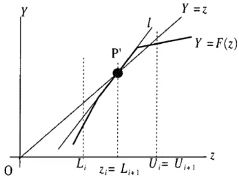
1 and valML(fd = L.

Proof: Figure 1 shows two cases (i)+(ii)(b) and (i)+(ii)(c), where C(9;) and C(96) are the slopes of two lines IL with a point

Pi

(L, valNL

(A,)) and lu with a point Ps(U, valv,,

(fu))

,

where (i)+(ii)(a) will be seen in Figure 2. We only prove (i). Initially, suppose that the algorithm does not stop during Step 1. Then the invariant (i) is satisfied from (4) of Step 1 and proposition 2.1. Note that we may assume C ( 6 ) = 0, though C(0;) may not be able to be determined uniquely. While the repeat statement (9)-(22) continues in Step 2, U is updated a t (19) only. So, we have (i).

Figure 1: Cases (i)+ (ii) (b) and (i)+(ii) ( c ) of Proposition 4.1

optimal flow in network

N .

If the algorithm does not stop during Step 1 then the value of the flow is contained in [L, U] at the end of the step. This observation is preserved during Step 2 while the length of interval [L, U] is cut in half.

Proposition 4.2: Let Li and Ui be a lower and an upper bounds at the beginning of z-

th repetition of the repeat statement (9)-(22) of Step 2, where Ll and Ul are the values obtained at the end of Step 1. Then we have for each z

(i) Ui+l - L. _{z+ 1} = Ui - ₂Li _'

(it) If there is the value 2" of an optimal flow in

N ,

then z* E [Li, Ui].

Proof: When we prove (ii), we show that z* ? [Li+l, U1+l] assuming z* E

[b,

Ui]. We have seen that (ii) holds for i = 1. Let z

=

z, = uliL1- a t the beginning of i-th repetition of the repeat statement. First, we consider the case when valNzG (fzi) = zi. We devide this case into the following two cases:

Case 1.1 (C(6zi)

<

1) : From proposition 2.3, we see that zi is optimal.

Case 1.2 (C'(6Zi)

>

1) : From proposition 2.3 and (14) of Step 2, we have z* _{[zi, Ui]} =

[Li+l, Ui+\}. Hence, we have Ui+i-Li+l = U--z- ~t = Ui-L. . See Figure 2, where P1(zi, valNz, (f,,))

is the intersection point of Y = z and Y = F{z).

Next we consider the case when valN,.(fz,)

#

Zi. Moreover, devide this case into the following two cases:

Case 2.1 (valNzG (f,,)

<

2,) : From proposition 2.3 and (19) of Step 2, if C(6;i)

<

1 and there is an optimal value z* then z* 6 [Li, zi) = Ui+l], which implies (i). For C(9;) = 1, we have no optimal flow in

N.

Otherwise(C(@;,)

>

l ) , an optima.1 flow in N , if exists, can not belong to [Li, zi], i.e. z* E [Li+l, Ui+l]. We also have (i) in this case.

Case 2.2 (valNzi (fzi)

>

zi) : We can see (i) and (ii) similarly. 0

Figure 2: Case 1.2 in the proof of Proposition 4.2

In the following we describe the way to calculate potentials <(v) (v E V). Given network

Afz

with a specific value z, find a generalized maximum flow

f,

a t first. Then let Tz be a subgraph of the residual graph G( fz) induced by the vertices that can reach the sink

t

by using the (residual) arcs of A( f,). From theorem 2.5,

G(

f,) has no generalized augmenting paths. So, there exist no flow-generating cycles in G( f,). Consequently, the canonical labels pz(v) (v ? V) are well-defined and can be computed by a Bellman-Ford shortest path algorithm with length

wz

(a)

=

- log

f ^

(a) (a E A(Tz)). Let P, be such a shortest

Generalized Balanced Flow Algorithms 169

path from v to t for each v E V(T,). Then we have ~ ( v ) = 2w2(pu) (v 6 V(T,)), where w,(Pv) = '^.aeA(Pv} w,(a). After the shortest path computation, we have p,(v) (v E V) satisfying that p-,(%a)

>

q z ( a ) u à £ ( 9 + a for each a E A(f,), where p,(v) is defined as ca for each v ? V - V(T,). The following proposition shows a relation between p, and

v

'

.

Proposition 4.3: The potentials T T ~ can be obtained by xi(v) = (v E V), where we

P': (v)

define <(v) = 0 for each v with p,z(v) = oo.

The following proposition states that the denomina.tor of each nonzero rational potential v'(v) (v 6 V - {s, t}) might be as big as r l , where

rl

=

n a g A ( ~ o ( a ) ~ l (a)).

Proposition 4.4: Each nonzero value of <(v) (v

s

V(T2)) is an integral multiple of F l l and bounded by F l , where

Tz is defined above. So are Oz(a) (a

? A).

Proof: For each v ? V(T,), let Pv be a simple shortest (directed) path from v to t of the residual graph G(fz) with length w,(a) s - log 'y^(a) (a E A(f,)). We can find such a simple path efficiently. Note that P, is also a highest gain residual path from v to

t

of G( f z ) with a gain ?fz(a) (a A( f,)). From proposition 4.3, a v ) is expressed as

where ii is the reverse arc of a. This means that xi(v) is an integral multiple of I',' and bounded by Fi. Next, we determine the values of 6*(a) ( a E A ) . Choose any arc a E A and assume u,(a)

>

0. If a A(f,), then from a

#

A(Pa-a), @*(a)

=

(-v;(a+a)

+

:'^i21~*(8a)]+

i i W z and irz

2

0, $;(a) is an integral multiple of F l l and bounded by Fl for

*

<

1, which implies

6^{d)

>

0. Otherwise, ii ? A(f,). From theorem 2.5 we have To(aln;(a+a) -

-7r; (@a)

+

3%;

(%a)

2

0. Hence we have this proposition.

From proposition 4.4 and integrality of u and

/?

we have

Proposition 4.5: For any z

2

0, D(6;) (resp. C ( 0 3 ) 2s an integral multiple of

r i l

(resp. (F1ra)-') where F2

=

naaai

(a).

Let

Li

and Ui be a lower and an upper bounds a t the beginning of z-th repetition of the repeat statement of Step 2 for 2

>

1. Consider an intersection between Y = z and a line with a slope C(Oci) passing through a point (Ui, valNu. ( fui )). The line is F ( z ) = C(O[,)z+ D(0&).

D(@&.

From proposition 4.1, the intersection is well-defined and is (z[, z',) with z[ = . Let

Proposition 4.6: If H ( z 9

>

0 and any one of the following conditions are satisfied during step 2, then we have

Ui

-

L,

2

rife;.

(i)Li

<

( f L i )

,

(22)

Li

= ( f t , ) and C(OL,)

>

1,

(222,)

Li

>

valfi, (fLi )

,

C

(Ok

)

>

1, 2:

2

Li

and

H

(za

5

Ui

-

Li

.

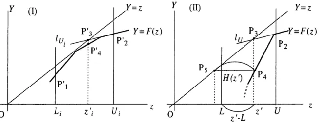
Proof: Note that these conditions (i)-(iii) correspond to (ii) (b), (ii) (c) a.nd (ii) (a) in proposition 4.1, respectively. The left graph (I) of Figure 3 shows a situation of (iii), where

we have

From proposition 4.5, H ( 4 ) is an integral multiple of

( r ~ r ~ r 1 r z

- J ) ) l for some integer

J (0

<

J

<

F i r a ) . Any case of the above conditions (i)-(iii) satisfies

U,

-

Li

2

ff(z,'). Note H(z[)

5

z; -

Li

for cases (i) and (ii), because val^, (f,;) = 2; - H(zi) and Y = F ( z )

2 1

is nondecreasing. So, we have Ui - Li

>

( F ; I ' j ) l

2

n;^-.

Suppose that we have reached Step 3. If H(z1)

>

0, then from proposition 4.6 we only have the invariant (i)+(ii)(a.) with z'

<

L or H ( 2 )

>

U - L. If H(z') = 0, then we have an optimal flow f z r in Af from proposition 4.1. Assume H ( 2 )

>

0. If z'

<

L,

then we see that

Af is infeasible. The remaining case is as follows: H (2')

>

U

- L, L

>

valAr, (ft), C ( @ i )

>

1 and z'

>

L.

Proposition 4.7: If H(zt)

>

U - L. L

>

valNL (fL), C(0;)

>

1 and z' _{L after (21) of}

Step 3, then we have no optimal flows in network Af.

Proof: From

H { z l )

>

U - L and U _-

>

zf we have z' _- - L

<

H(zi). Consider the right graph (11) of Figure 3, where we have P a p 4 = P4P5 =

H(zt).

We can not find any optimal solutions in the region of a triangle PsP4P5.

Figure 3: Situations (I) and (11) of Propositions 4.6 and 4.7

In order to compute an optimal flow in

Afz

in Steps 1 ~ 3 we will use one of efficient algo- rithms for the generalized maximum flow problem. Such two examples are Iterative Fat-Path

Algorithm by Radzik

[lo]

and Highest-Gain Augmenting Path Algorithm due to Goldfarb,

Jin, and Orlin [4]. The former is a best known combinatorial approximate algorithm, while the latter is a best known combinatorial exact one with 0 ( m 2 ( m

+

n logn) log B'), where

B' is the largest integer used to represent the gains and capacities in the network. We take

up the former ,here. His algorithm repeatedly cancels flow-generating cycles for finding an e-optimal flow in network

Aft

= (G,

u,

7, s, t) with a given e (1

>

e

>

0). A generalized flow

f

in

At'

is e-optimal if valNi (f I ) - valNr ( f )

<

e valN (f ') for some generalized maximum

flow f t in Aff. The next lemma from [11] indicates that if a generalized flow is e-optimal for sufficiently small e, then it is essentially optimal.

Generalized Balanced Flu w Algorithms 171

L e m m a 4.8: Let f be a B'3'n-optimal flow in network A/"'. T h e n we can compute a n optimal flow in

N'

in 0(mnmin{rn, n log B'}) time, where 0 is the complexity deleting a factor polylogarithmic i n n and B' = m a . ~ ~ ~ ~ { m a x { 7 ~ ( a ) , yi (a), " ( a ) } } .

The description of his algorithm is as follows where we wll omit the details here.

Iterative-Fat-Path-Algorithm(Af', e):

A

-

Ao;

f + 0, where 0 is zero flow in

At';

while A

>

e valN/ ( f ) d o

b e g i n

(h, p ) ^- Cancel-Cycles (N'(

f )

,

&

) ;

f + f

+ A ;

f t Remove-Cycles ( f ) ;

?(a) + - for each (residual) arc a of

A/"'(');

ij +- F a t A u g m e n t a t i o n ( ( G ( f ) , u f ,

T),

&); g +- Interpretation(g}\

f

^ f

+ g ; A - 4 - _{2 '} e n d ; r e t u r n f ; 0

In this algorithm, we can choose A. as any value satisfying

fi-11

$ valNI(f1) $ A0 for some optimal flow f f in A/"'. Moreover, procedures not defined are as follows. Can-

cel-Cycles(A/"', e) returns a pair (A, p ) of a pseudoflow A with fl,/i(v)

<

0 (u

e

V) and a labeling p such that %(a)

5

1

+

e for each a of .A/"'(h) where a pseudoflow h in

A/"'

is a function h : A + R+ satisfying (2.2). Remove-Cycles(f) repeatedly finds and deletes a flow-generating cycle flow from f , and returns the final pseudoflow without such cycle flows. Fat-Augmentation((G( f

),

uf,

Â¥:I)

&) finds a pseudoflow ij in (G( f ),

u!,

7)

such that I ~ a l ~ < ; ( ~ ~ , ~ ~ , - , ) (9') - valjc; jl,u;,q) (ij)l for some optimal flow g' in (G( f ), u f ,

q).

I n t e r p r e t a t i o n ( 3 ) returns a function g : A -+ R+ such that g is equal to ij as a function

restricted on A(f) but is interpreted as a pseudoflow in

At'.

Concerning the complexity of the above algorithm, the following facts (i) and (ii) are known from [lo]: (i) The run- ning time of one iteration of the while statement is 0 ( m ( m

+

n log n log(: log B'))) where B' = maxaEA {max{'yo(a), (a), u(a) }} ; (ii) There are at most O(1og

9

iterations. We summarize the total complexity as a theorem.

T h e o r e m 4.9:

PO]

Iterative Fat-Path algorithm computes a generalized maximum flow of network

N'

in 0 ( m log a ( m

+

nlog n log(: log B')) time. D

From theorem 4.9 and lemma 4.8, we can find an optimal flow in network

JV

in O(m2(m

+

m n log n log B') log 5 ' ) time. Now we show the total running time of our algorithm:

T h e o r e m 4.10: Our binary search algorithm runs in O(m log B M{n,

m,

B')) time, where

B = max{B1, B"} for B', B" in OUT algorithm, and M(n, m,

BF)

denotes the complexity of

solving a generalized m a x i m u m flow problem i n a network with n vertices, and m arcs, and nonnegative capacities and gains expressed as integers between 1 and

B'.

Proof: We use Bellman-Ford shortest path algorithm to compute IT'. Such a shortest path

computation takes O(nm). From O(nm+M(n, m, B')) = O(M(n, m, B')), Steps 1 and 3 run

1 72 A. Nakayama & C.-F. Su

k of repetitions of the repeat statement in Step 2 satisfies

<

&.

Each repetition takes

M(n, m ,

B'}

time. From B

>

B',

we have this theorem.

a

We present an example in the following.

Example: An instace

Af

has G with V = {s, x, y, t} and A = {(s, x), (s, y), (x, y), (x, t ) , (y, t)}. A triple (u(a), ~ ( a ) , &(a)) for each a E A is given by (s, a:) : (8,

$,

j),

(s, y) : (5,

$,

$),

(x, y) : (2,

i,

j ) , ( x , t ) : (1,

3,

$), (y, t) : ( 4 , 2 , $ ) where

/3

= 0. Then we have B = B' = 8. Apply our algorithm for this instance. At the end of Step 1, we have U = 2 x 64 = 128 and

L = 0 and go to Step 2. After the fifth iteration of the repeat statement in Step 2, we have

1 14 1

L = 4 and U = 8. Continuing these processes, we have L = - and U = 7

+

after Step 2. Finally, we get the optimal value z* = during Step 3.

The second algorithm uses the parameterized search technique of Megiddo instead of our binary search in addition to one of efficient algorithms for finding generalized maximum flows. The reasons for proposing the second algorithm are as follows. If B' is sufficiently smaller than

B",

then it is possible that the second algorithm is faster than the first one where B', B" are defined in Step 1 of the first algorithm. Moreover, it can be regarded as a generalization of a parameterized algorithm given by Zimmermann [12]. We briefly explain the second algorithm because the analysis is quite similar to Zimmermann's. Choose an efficient algorithm A for the generalized maximum flow problem. Note that it is easy t o test feasibility of the generalized maximum flow problem, because lower capacities are zero in our model. Each step of the algorithm

A consists of additions, scalar multiplications, and

comparisons. We use the algorithm

A

to obtain a generalized maximum flow in network

Nt,

where this generalized maximum flow contains z as a parameter. Each scalar value p considered by the algorithm corresponds to a linear function p

+

zq for some scalar q in the parameterized problem. Instead of adding p

+

p' for another scalar p', we add linear functions (p

+

zq)

+

(p'

+

zq'), where q' is a scalar. If we compare p

+

zq with p'

+

zq', then we need to know the critical value z" determined by p

+

zq = p'

+

zq' unless q = q'. Then we can decide whether z >, z" or z

<

z" by running the algorithm

A for network NZ". In

our case, add a super sink t' and an additional arc (t.

t')

to network N z . Define uz(t,

t')

= z

and ~ ( t , t') = a ( t , t') = 1. Let

A/"

be the enlarged network. Suppose that network

Jf;,

is feasible. If (t, t') is saturated then we have z

2

z". Otherwise, we have z

<

z". We say that (t, t') is saturated if the flow value of (t, t') is equal to az (t, t'). In the case when is infeasible, we have z

>

z". With that information in hand, we can work the algorithm A for the parameterized problem A/*. Finally, we get a generalized maximum flow fz in network

x .

If (t, t') is not saturated, then there exists no generalized maximum balanced flow in N . Otherwise, the optimal value is z* = minaeA za, where Za = max{z : 0

<

f z ( a )

5

az(a)} for each a ? A.

If we use a highest-gain augmenting path method in the second algorithm, then we have

Theorem 4.11: The second algorithm runs in O({'mP(m

+

n log n ) log B'}2) time, where

B'

= m a x a ~ A { ' m a x { ~ ~ (a) TI (a), u{a) )

1 .

5. Conclusions

As a new generalization of the maximum bala,nced flow problem considered by Minoux, we gave the generalized maximum balanced flow problem and proposed two efficient algo- rithms. One of future researches is to consider our model with nonzero lower ca-pacities l(a) (a E A). Though we can analyse the model with ((a) ( a E A ) in the sa'me way as in this paper, we must solve a feasibility problem, i.e. a problem of testing whether there is a feasible generalized flow in the underlying network with l(a) ( a E A). The authors believe

Generalized Balanced Flow Algorithms 1 73

that this feasibility problem is open. On making our algorithms strongly polynomial even if l(u) = 0 (a E A ) , there is an obstacle which is another open question of answering whether it is possible to solve the generalized maximum flow problem in strongly polynomial time.

6. Acknowledgn~ent

We would like to express our thanks to Professors Satoru Fujishige) Kazuhisa Makino, and Takeshi Takabatake of Graduate School of Engineering Science, Osaka University for useful commemnts. h4y sincere thanks are also due to two anonymous referees for pointing out not a few errors in) and suggesting many improvements) to the original version of our paper.

References

[I] W.-T. Cui:

A

network simplex method for the maximum balanced problem. Joarnal of the Operations Research Society of Japan, 31(1988) 551-564.

[2] L. R. Jr. Ford and D. R. Fulkerson: Flows in Networks. (Princeton University Press. Princeton,

N.

J., 1962).

[3] S. Fujishige, A. Nakayama and W.-T. Cui: On the equivalence of the maximum bal- anced flow problem and the weighted minimax flow problem. Operations Research Let- ters, lti(1986) 365-376.

[4] D. Goldfarb, Z. Jin, and J. B. Orlin: Polynomial-time highest-gain a,ugmenting path al- goritl~ms for the generalized circulation problem. Mathematics of Operatzons Research, 22(1997) 793-802.

[5] T. Ichimori, H. Ishii and T. Nishida : Weighted minimax real-valued flows. Journal of the Operations Research Society of Japan, 24(1981) 52-60.

[GI N. h4egiddo : Combinatorial optinlization with rational objective functions. Mathemat- zcs of Operations Research, 4(1979) 414-424.

[7] h4. Minoux: Flots kquilibrks et flots avec skcuritk. E.D.F.-Bullentin de la Direction des ~ t u d e s et Recherches, Skrie C-Mathkmatique, Infomatique, l(1976) 5-16.

[8] A. Nakayama: A polynomial algorithm for the maximum balanced flow problem with a constant balancing rate function. Journal of the Operations Research Soczety of Japan, 29 (1986) 400-410.

[9] A. Nakayama: A polynomial-time binary search algorithm for the ma.ximum balanced flow problem. Joarnal of the Operations Research Society of Japan) 33(1990) 1-11. [lo] T. Radzik : Faster algorithms for the generalized network flow problem. Mathematics

of Operations Research, 2 3 (1998) 69- 100.

[I 11 K. D. Wayne: Generalized h4aximum Flow Algorithms, Ph. D. thesis) Cornell University, 1999.

[12] U. Zimmermann: Duality for balaaced submodula,r flows. Discrete Applzed Mathemat-

ZCS) 15 (1986) 365-376.

Akira Nakayama Chien Fei Su

Faculty of Administration and Social Sciences President: Tokuritsu Co. Ltd.

Fukushin~a University 318-1 Nishiyajinla, Ohta, Gumma)

1 Kanayagawa, Fukushima, 960-1296 Japan 373-0823 Japan