Investment Behavior and Business Sentiments of Small and Medium Enterprises
著者 MATSUSHIMA Shigeru, TAKECHI Kazutaka
出版者 Institute of Comparative Economic Studies, Hosei University
journal or
publication title
Working Paper
volume 144
page range 1‑22
year 2009‑01‑21
URL http://hdl.handle.net/10114/4003
Investment Behavior and Business Sentiments of Small and Medium Enterprises ∗
Shigeru Matsushima
†Kazutaka Takechi
‡January 21, 2009
Abstract
This paper uses survey data to investigate how subjective perceptions of business con- ditions affect the investment behavior of small and medium enterprises (SMEs) in Japan.
Using panel data, we show that while positive perceptions of business conditions induce investment, long-term improvements in business conditions are required for manufactur- ing firms to invest. We also find that perceptions of financial conditions affect investment:
firms invest if it is easier to borrow money and if interest rates are lower in the current period. However, if firms expect a decrease in future interest rates, they may delay invest- ment and are unlikely to invest in the current period. Finally, firms suffering a shortage of labor are likely to invest. This is because unlike large firms, SMEs may face some difficulty in employing the labor force required, and thereby substitute capital for labor.
∗We would like to thank Yuji Genda and seminar participants at Hosei University and the Small and Medium Enterprise Agency. Any remaining errors are our own. Financial support for this research was provided by a Grant-in-Aid for Scientific Research by the Japan Society for the Promotion of Sciences (No.18730175 (Takechi))
†Graduate School of Management of Science and Technology, Tokyo University of Science
‡Faculty of Economics, Hosei University. Email: [email protected]
1 Introduction
Firm investment is a major driving force of economic growth and business cycles. Thus, an im- portant issue is the examination of what determinants of real investment are significant. In the macroeconomics literature, the investment decision is considered to be based on fundamentals, including capital adjustment and profitability shocks (for example, Lucas and Prescott (1971) and Hayashi (1982)). In this study, we emphasize that subjective factors are also fundamental elements for investment decision making. That is, firms with pessimistic perceptions may be less likely to invest than otherwise. We address this issue by considering the kinds of subjective factors that determine investment behavior.
This paper analyzes the investment behavior of small and medium enterprises (SMEs) us- ing panel data collected by the Organization for Small and Medium Enterprises and Regional Innovation, Japan (SMRJ). We focus on the relationship between the perception of firms about their own business conditions and real activity in the form of investment. The data source contains various types of perceptions held by SMEs of business conditions, financial condi- tions, and the level of production facilities. The SMRJ undertakes the survey by administering questionnaires to SMEs about their business sentiments and investment decisions. The survey questions include ”whether the business conditions of your firm are better offthis year than last year?”, ”whether the business conditions of your firm are good in the current period?”, and ”whether you have invested in the current period?” Using this information, we construct dummy variables for business sentiments and investment decisions to identify the link between them.
Unlike large companies, it may be reasonable to consider that the investment decisions of SMEs are associated with the discretion of their owners. In large companies, the investment decision is affected by their organizational form and company rules governing the determina-
tion of investment. Therefore, there may not be a close relationship between business senti- ments and investment activities. In contrast, owners of SMEs may have some discretionary power over the investment decision. Therefore, there could be a close relationship between en- trepreneurship (or animal spirits) and investment. Using data on SMEs enables us to analyze whether this relationship exists.
In the finance literature, studies have been undertaken concerning the predictability of busi- ness sentiment on financial investment returns (Wang (2003)). In addition, business or investor sentiment is considered as an important factor for mispricing, excessive responses to informa- tion, and excessive volatility in stock markets (for example, Barberis, Shleifer, and Vishny (1998) and Dumas, Kurshev, and Uppal (2005)). In the psychology literature, these phenom- ena are consistent with the finding that individuals do not respond excessively under uncer- tainty (conservatism, Edwards (1968)) and treat specific events as general (representativeness, Tversky and Kahneman (1974)). While these studies reveal the importance of psychological factors and their effects on financial investment, there are no known studies concerning their effects on real investment. While the relationship between business sentiments and real eco- nomic activity is considered using aggregate consumption (Acemoglu and Scott (1994)) and micro data (Hayashi (1985), Jappelli and Pistaferri (2000), and Souleles (2004)), these studies investigate consumer sentiments, not firm sentiments. This may be due, in part, to data lim- itations. To our best knowledge, there is no extensive study using the sentiments of business managers. Because investment has a large impact on business cycles and growth, it is im- portant to investigate the effect of the psychological factors held by business managers. This study contributes to the literature by identifying the particular psychological elements that are significant.
As the financial data available on SMEs is not sufficient, we are unable to construct an
index of fundamental value (like Tobin’s Q). Instead, we explore the panel data characteristics by assuming that firm fundamentals are firm specific and do not change over time. We are then able to use the data on firm perceptions of the difficulties in fund raising, changes in the interest rate faced, and whether a firm has a shortage or excess of labor. We examine whether these elements are significant in the investment decision.
We find that if managers perceive the status of business conditions as being good, they tend to invest. In addition, in manufacturing firms, if business conditions are better offin two con- secutive periods, the probability of investment increases. Therefore, at least for manufacturing firms, investment is based on improvements in long-term business conditions. With respect to financial conditions, if firms consider that financing has become easier and if interest rates fall relative to the previous period, investment is more likely to take place. Because we found that future expectations of falls in interest rates have a negative impact on current investment, firms decide whether to invest in a forward-looking manner. We also find that if firms consider that the firm is short of labor, they tend to invest. This reflects the fact that it is difficult for SMEs to find employees, even if they demand more labor, so they substitute capital for labor. These findings help illustrate the basic nature of investment behavior by SMEs.
This paper is organized as follows. Section 2 introduces the data set. In Section 3, we describe our empirical framework. Section 4 provides the empirical results. The final section concludes.
2 Data
The data employed is survey data collected and compiled by SMRJ and the Research Institute of Social Science at the University of Tokyo. The survey data is from a questionnaire of business sentiments and investment behavior. The data also contains other firm information,
such as the number of employees, the firm’s industry, and the prefecture where it is located.
We link the responses for business sentiments and investment.
The sample period is from 1998 to 2006. While SMRJ obtains the data on a quarterly basis, only the April–June (first quarter) data is used to construct the panel data. Therefore, the results obtained in this study should be treated with some caution as we do not take into account investment in other periods. We have data from 4,439 firms, including not only the manufacturing sector, but also the wholesale, retail, service, and construction sectors. For the manufacturing sector, there are 1,422 firms. The questions range widely, and include business conditions, changes in the number of employees, financial conditions, production facilities, and investment decisions. For example, with respect to business conditions, the question is
“compared with the last same period, your firm’s business condition is (1. better off), (2.
unchanged), (3. worse off).” The question about investment is “whether you invest in this period?” and the choices available are “(1. yes), (2. no).”
We construct dependent and independent variables using the survey data. Because the data on investment is discrete (yes or no), the investment decision is treated as a discrete choice.
We denote the investment decision by firm i at period t by:
Yit=
1 if invest 0 otherwise
This is our dependent variable. The main explanatory variables are dummy variables express- ing psychological factors. There are two types of business condition perceptions: changes and levels. We construct the variables as follows. DBetterL takes a value of 1 if firms respond that business conditions are better from the same period last year, otherwise 0. The same period last year means that, for example, business conditions in the first quarter of 2001 are compared
with the first quarter of 2000. DWorseL takes a value of 1 if firms respond that business con- ditions have worsened from the same period last year, otherwise 0. For levels, DGood takes a value of 1 if firms respond that the level of business conditions are good, otherwise 0. DBad takes a value of 1 if firms respond that the level of business conditions are bad, otherwise 0.
The variables are shown in table 1. In addition, in order to consider long-term changes in busi- ness conditions, we construct a two-period consecutive improvement and worse offmeasure.
These are shown in table 2.
Table 1: Business Sentiments
Variables Explanation
DBetterL 1 if better offthan the same period last year; otherwise 0.
DWorseL 1 if worse offthan the same period last year; otherwise 0.
DGood 1 if current business conditions are good; otherwise 0.
DBad 1 if current business conditions are bad; otherwise 0.
Table 2: Business Sentiments 2
Variables Explanation
DBetter2L 1 if better offfor two consecutive years; otherwise 0.
DWorse2L 1 if worse offfor two consecutive years; otherwise 0.
These variables are sufficiently rich to capture the perceptions of business managers of the business conditions their own company faces. They then can be considered as important factors affecting investment decisions. In addition, the survey data contains firm responses concerning perceptions of the input side of investment or aspects of financing. For the difficulty of obtaining long-term debt, LtermDebtEasy takes a value of 1 if the manager responds that financing is easier than the same period last year, otherwise 0. Similarly, LtermDebtHard takes
a value of 1 if the manager responds that financing is more difficult than the same period last year, otherwise 0. In addition, we account for the expectations of managers. ELtermDebtEasy takes a value of 1 if the manager responds that the firm will find financing easier in the next period, otherwise 0. ELtermDebtHard takes a value of 1 if the manager responds that it will be harder for the firm to obtain financing in the next period, otherwise 0. The finance variables are shown in Table 3.
Table 3: Financial Aspects 1
Variables Explanation
LtermDebtEasy 1 if easier than the same period last year; otherwise 0.
LtermDebtHard 1 if more difficult than the same period last year; otherwise 0.
ELtermDebtEasy 1 if prospects for the next period are easy; otherwise 0.
ELtermDebtHard 1 if prospects for the next period are easy; otherwise 0.
The survey also enables us to construct variables for interest rate perceptions. These are not objective in the sense that the interest rate referred to is not the actual market interest rate, rather the rate firms consider they face when they borrow money from financial institutions.
With respect to interest rate changes, IrateRise takes a value of 1 if the manager responds that interest rates have risen from the same period last year, otherwise 0. IrateFall takes a value of 1 if the manager responds that interest rates have fallen from the same period last year, otherwise 0. Finally, the survey includes responses to a question on expectations of interest rates. EIrateRise is the index of rise of the expected interest rate in the next period and EIrateFall is that of fall of the expected interest rate. Table 4 details the variables.
Finally, we take into account the situation where managers decide to invest so as to adjust their optimal level of capital and labor. This data is only available for manufacturing firms.
OptFactoryEx takes a value of 1 if the manager responds that there is excess production ca-
Table 4: Financial Aspects 2
Variables Explanation
IrateRise 1 if the interest rate has risen from the same period last year; otherwise, 0.
IrateFall 1 if the interest rate has fallen from the same period last year; otherwise, 0.
EIrateRise 1 if the next period interest rate is expected to rise; otherwise 0.
EIrateFall 1 if the next period interest rate is expected to fall; otherwise, 0.
pacity, otherwise 0. OptFactoryShort takes a value of 1 if the manager responds that there is a shortage of production capacity, otherwise 0. Similarly, OptEmplyEx takes a value of 1 if the manager responds that there is an excess of labor, otherwise 0. OptEmplyShort takes a value of 1 if the manager responds that there is a shortage of labor, otherwise 0. By considering these factors, we are able to examine whether managers adjust their production facilities to their psychologically optimal level. Table 5 presents these variables.
Table 5: Optimal Size of Labor and Capital
Variables Explanation
OptFactoryEx 1 if production facilities are in excess; otherwise 0.
OptFactoryShort 1 if firms are short production facilities; otherwise 0.
OptEmplyEx 1 if the number of employees is in excess; otherwise 0.
OptEmplyShort 1 if firms have a shortage of labor; otherwise 0.
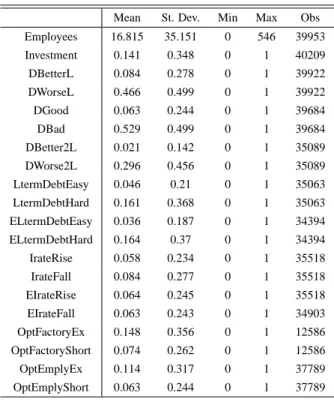
Table 6 provides summary statistics for our data. This table presents statistics of the vari- ables denoted above and the number of employees. The average number of employees in our sample firms is about 17; the maximum is 546 employees. The average investment of 0.141 indicates that about 14 percent of firms invest on average. While only about 8 percent of firms respond that business conditions are better than the previous year, about 47 percent of firms consider themselves worse off. These indicate that business performance worsens, on average,
for SMEs in our sample period. Similarly, the percentage responding that it becomes more difficult to obtain finance is about 16 percent, while only about 6 percent of respondents find financing easier. There is not much difference between the interest rate changes, with about 6 percent responding that interest rates have risen and 8 percent responding that they have fallen.
Finally, in 11 percent of firms the number of employees is considered excessive, while 8 per- cent of managers respond that they face a shortage of labor. Because not all firms respond to all questions every year, the data forms an unbalanced panel.
Table 6: Summary Statistics
Mean St. Dev. Min Max Obs
Employees 16.815 35.151 0 546 39953
Investment 0.141 0.348 0 1 40209
DBetterL 0.084 0.278 0 1 39922
DWorseL 0.466 0.499 0 1 39922
DGood 0.063 0.244 0 1 39684
DBad 0.529 0.499 0 1 39684
DBetter2L 0.021 0.142 0 1 35089
DWorse2L 0.296 0.456 0 1 35089
LtermDebtEasy 0.046 0.21 0 1 35063
LtermDebtHard 0.161 0.368 0 1 35063
ELtermDebtEasy 0.036 0.187 0 1 34394
ELtermDebtHard 0.164 0.37 0 1 34394
IrateRise 0.058 0.234 0 1 35518
IrateFall 0.084 0.277 0 1 35518
EIrateRise 0.064 0.245 0 1 35518
EIrateFall 0.063 0.243 0 1 34903
OptFactoryEx 0.148 0.356 0 1 12586
OptFactoryShort 0.074 0.262 0 1 12586
OptEmplyEx 0.114 0.317 0 1 37789
OptEmplyShort 0.063 0.244 0 1 37789
Year 1998-2006
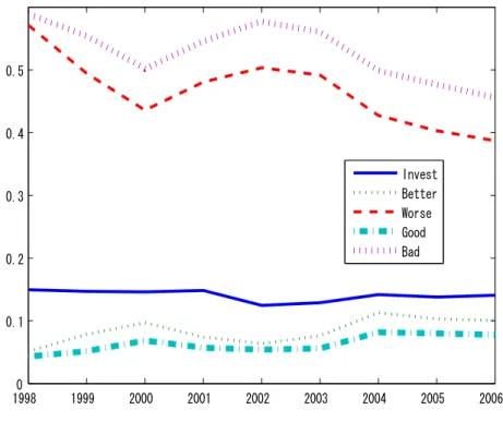
In order to have a basic idea about the time series changes of these variables, we plot the av- erage values in each year. Figure 1 shows the investment probability and business conditions.
“Invest” is the percentage of firms investing, “Better” is firms indicating DBetterL, “Worse” is firms indicating DWorseL, “Good” is firms indicating DGood, and “Bad” is firms indicating DBad. These show that when business conditions are better or good, the probability of invest-
19980 1999 2000 2001 2002 2003 2004 2005 2006 0.1
0.2 0.3 0.4 0.5
Invest Better Worse Good Bad
Figure 1: Business Sentiments and Investment
ment increases. It also suggests that there is a lagged effect when considering the relationship between 2000 and 2002. In 2000, the percentage of firms considering business conditions good or better increased, with the number of firms investing increasing one year later in 2001.
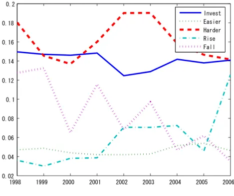
Figure 2 shows the relationship between finance and investment. “Easier” is the percentage of firms indicating LtermDebtEasy, “Harder” is firms indicating LtermDebthard, “Rise” is firms indicating IrateRise, and “Fall” is firms indicating IrateFall. These relationships imply that there could be a negative relationship between financial difficulty and investment. For instance, when the percentage of firms finding finance more difficult increases, the percentage of firms with investment decreases. However, we cannot find a clear relationship between investment and interest rates using the figure.
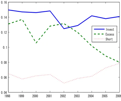
Finally, Figure 3 shows the relationship between labor shortage/excess and the investment decision. “Excess” is the percentage of firms indicating OptEmplyEx and “Short” is firms indicating OptEmplyShort. This figure shows that from 2000 to 2002 the percentage of firms
1998 1999 2000 2001 2002 2003 2004 2005 2006 0.02
0.04 0.06 0.08 0.1 0.12 0.14 0.16 0.18 0.2
Invest Easier Harder Rise Fall
Figure 2: Financing and Investment
considering that labor is in excess increases and the investment percentage decreases. From 2002 to 2006, while the percentage of excess labor decreases and the percentage of firms short of labor increases, the investment percentage increases. This relationship will be examined in the empirical section to obtain the implications for labor–capital substitution.
In the next section, we empirically examine the effects of firm perceptions of business and financial conditions on investment behavior.
3 Empirical Framework
We set up an empirical framework to study the investment behavior of SMEs. Because our data on investment is whether a firm invests or not, we employ a discrete choice model (for discrete choice investment model, see Adda and Cooper (2003)). The investment choice variable of
1998 1999 2000 2001 2002 2003 2004 2005 2006 0.04
0.06 0.08 0.1 0.12 0.14 0.16
Invest Excess Short
Figure 3: Optimal Size and Investment firm i in period t is given by:
Yit =
1 if invest 0 otherwise.
The manager’s problem is to maximize the expected sum of future discounted profit:
maxYi
E X
t
π(Yit,Xit),
where Yi = {Yit}t, Yit = {invest,not invest}, Xit is the state and exogenous variables asso- ciated with profit. The Bellman equation is expressed by V = max{Va,Vn}, where Vj = π( j,Xit)+ βEV(Yit+1,Xit+1), j = a,n, a corresponds to investment, and n to no investment.
In this study, instead of specifying functional forms and solving the dynamic programming problem explicitly, we employ a reduced form approach. That is, we denote W =Va−Vn and
consider a choice problem that if W is positive, a manager decides to invest. Therefore, the investment decision is expressed by:
Yit = I(Wit≥ 0),
where I(·) is the indicator function.
The variable, Wit, is affected by a variety of elements. As mentioned, we consider that the psychological elements of managers and firm-specific factors affect Wit. When we express business sentiments explicitly, Witis specified as follows:
Wit =β0+β1Sizeit+β2DBetterLit+β3DWorseLit+β4DGoodit (1) +β5DBadit+β6DBetter2Lit+β7DWorse2Lit+δXit+eit,
where Size is the number of employees, DBetterLit is the index of better business condi- tions from the last year, DWorseLit is the index of worse business conditions from the last year, DGooditis the index of good current business conditions, DBad is the index of bad cur- rent business conditions, DBetter2Lit is the index of two consecutive years of better business conditions, DWorser2Lit is the index of two consecutive years of worse business conditions, Xit are other covariates, and eit is the error term. In the following, we describe what factors, including financial aspects, are included in Xit.
For estimation, we employ a linear probability model: Yit = Wit. Because we do not have many firm characteristic variables, it is important to control for firm heterogeneity. We control for firm heterogeneity using fixed effect estimation. We also use time dummies to take into account any time-specific effects. These controls enable us to identity the relationship between investment and psychological factors. For a robustness check, we also employ conditional
logit estimation.
3.1 Difficulty in Finance and Production Facilities and Labor
The factors affecting Xitare financial aspects and production facilities/labor optimal levels. As many SMEs face financial constraints, they rely on debt finance to engage in real investment activity. Therefore, it is important to investigate the effect of these financial aspects. Our data includes perceptions of the difficulty of finance and interest rate changes. These variables are more appropriate than countrywide or regional interest rates because true financial conditions differ among firms. Hence, we reasonably consider that these perceptions held by managers have an impact on investment. The variables shown in Tables 3 and 4 capture the status of debt demand SMEs face in detail. Examination of the financial aspects and investment reveals the importance of these psychological factors.
Finally, for firm characteristics, Xit, we consider the aspects of production facilities and labor. For manufacturing firms, there is data on whether the current production facilities and the number of employees is optimal. We introduce dummy variables associated with the excess and shortage of production facilities and labor. The relationship between investment and these variables shows how firms adjust their production capacity. Thus, our survey data enables us to examine the effects of a variety of psychological factors (business sentiments, financial conditions, and production capacities) on real investment.
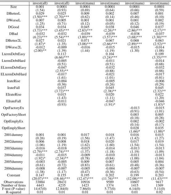
4 Estimation Results
Table 7 reports the results of the panel fixed effects estimation. Columns 1 and 2 show the results using data from all industries. Columns 3 to 6 report the results using manufacturing firms only. The result using only the business conditions variables are reported in Columns 1
and 3.The remaining columns show the results including the financial or production facilities factors.
From Columns 1 and 2 in Table 7, we find that if business conditions are better off than in the previous year, the probability of investment increases. Column 1 also shows that when we employ only the business conditions variables, two consecutive years of better off and worse off business conditions affect the probability of investment positively and negatively, respectively. These results reveal the intuitive relationship between business sentiment and investment: firms considering their own business conditions as being better offare likely to invest and firms considering their own business conditions as worse offare unlikely to invest.
As both Columns 1 and 2 show, the levels of business conditions significantly affect invest- ment. Therefore, our results suggest that improvements in business conditions and the level (not change) of business conditions are important for investment.
Column 2 reports the results using the financial aspects. While the results are similar to Column 1, the insignificance of long-term changes in business conditions (DBetter2L and DWorse2L) may be caused by including firms across all industries. Because real investment is more important for manufacturing firms than for other firms in other industries, we employ the same estimations using only the data on manufacturing firms.
Columns 3 to 6 report the results using the data on manufacturing firms. These show that while improvements in business conditions from the past year do not affect investment, the two consecutive years improvement increases the probability of investment. This suggests that for the manufacturing industry, the investment decision is based on long-term performance. This contrasts with the results using data from all industries, including wholesale, retail, service, and construction firms. Because investment in manufacturing firms means that firms purchase or develop production facilities, the scale of investment may be larger than in other industries.
These investment costs are sunk costs to some extent; therefore, they require a sufficient im- provement in business conditions to be able to invest. Note that because our data only covers the first quarter, the data coverage may bias the effect on investment. That is, as our data cannot capture investment in periods other than the first quarter, if improvements in business conditions affect investment in other periods, we cannot identify its effects. Nevertheless, the contrast between manufacturing and all industries reveals the specificity of investment in the manufacturing industry.
The subjective factors affecting investment include not only business sentiments, but also their financial aspects. Columns 2, 4, and 6 report the results using financial aspects. In all estimations, when it is easier to borrow money and the interest rate decreases, the probability of firm investment increases. These results suggest that easier financial conditions significantly affect investment behavior. Policies mitigating financial difficulties in SMEs will then promote investment because firm investment is sensitive to the perceptions of available finance.
Columns 4 and 6 show that expectation of a future interest rate decrease affects current investment negatively. This suggests that the investment decision of managers is forward- looking. Firms expecting future interest rate falls refrain from investing today and may delay investment until the next period. As expectation of a future interest rate increase does not cause an increase in current investment, the investment choice related to future interest rate changes is asymmetric. Put differently, it is less costly not to invest, therefore only interest rate increases have a significant negative impact.
Finally, Columns 5 and 6 report the estimation results taking into account the optimal level of capital and labor. The significant factor is where labor is in shortage. This suggests that firms with less labor from the optimal level increase the probability of investment. This may reveal the labor market conditions SMEs face. Because workers would prefer to obtain
employment in large firms, it is difficult for SMEs to assure their labor force. Hence, firms with an incentive to employ labor invest instead of hiring. This implies that substitution between labor and capital is conducted by firms with difficulties in hiring labor.
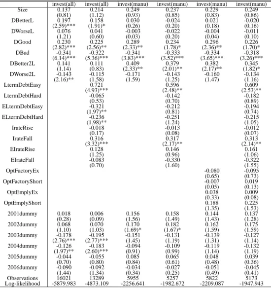
To check the robustness of our linear probability model, we also employ conditional logit estimation. Table 8 reports the estimation results of the conditional logit model. The number of firms included differs from the linear probability model because the likelihood of firms not investing in any period and investing in all periods is zero. These firms are excluded from the sample. The results are qualitatively similar to the linear probability models, thereby supporting the robustness of the results.
In summary, the significant factors are (sign in parenthesis indicates effect on investment):
• Business conditions better offfrom last year (all industries) (+)
• Business conditions better offfor two consecutive years (manufacturing) (+)
• Current business conditions are good (+)
• Current business conditions are bad (-)
• Debt finance easier than last year (+)
• Interest rates fall (+)
• Expectations of a future interest rate decrease (-)
• Shortage of labor (manufacturing) (+)
From these results, we show the kinds of factors related to investment behavior. The sig- nificant relationship between business sentiments and investment reveals the important effect of psychological factors on real economic activities. Because financial conditions and interest
rates significantly affect investment, the findings suggest the importance of financial policy.
Finally, the substitution between capital and labor suggests that SMEs face difficulties in en- suring an adequate labor force. This aspect is essential for analysis of the production structure of SMEs.
5 Conclusion
This study empirically investigates the connection between investment behavior and psycho- logical factors in Japanese SMEs. We use panel data on business sentiments and investment using a survey conducted by the SMRJ. Our findings reveal the importance of business senti- ments for investment decisions. In particular, with respect to changes in business conditions, long-term improvements have a significant impact on investment by manufacturing firms. We also find that the level of business conditions is important for the investment decision.
Factors other than business sentiments, such as perceptions of finance and production fa- cilities, also affect investment. If it is easier to debt finance and if interest rates decrease, investment is likely to occur. One interesting finding is that if expectations of the future inter- est rate suggest a decrease in rates, firms are unlikely to invest. This is because they may adopt a delaying strategy of waiting and investing in the next period. Finally, firms short of labor are likely to invest. This suggests that when firms are unable to obtain an appropriately sized labor force, they substitute capital for labor. This phenomenon may be particular to SMEs.
While our results can reveal the impact of psychological factors on investment choice by using business sentiments data of SME managers, we put forward two important issues requir- ing future research. The first is that the data included here covers only the first quarter and does not contain detailed financial data. Use of some complementary data with matching techniques (for example, Angrist and Krueger (1992)) may reduce any biases involved. The second con-
cerns the endogeneity of business sentiments in that business sentiment may be subject to past investment behavior. This can be potentially controlled for using instrumental variable (IV) or generalized method of moments (GMM) techniques. Both areas require future research.
References
Acemoglu, D., Scott, A., 1994 Consumer confidence and rational expectations: Are agents’
beliefs consistent with the theory? Economic Journal 104, 1–19.
Adda, J., Copper, R., 2003 Dynamic Economics, MIT Press.
Angrist, J.D., and Krueger, A.B., 1992 The effect of age at school entry on educational attain- ment: An application of instrumental variables with moments from two samples, Journal of American Statistical Association 87, 328–336.
Barberis, N., Shleifer, A., Vishny, R., 1998 A model of investor sentiment, Journal of Financial Economics 49, 307–343.
Dumas, B., Kurshev, A., Uppal, R., 2005 What can rational investors do about excessive volatility and sentiment fluctuations? NBER Working Paper 11803.
Edwards, W., 1968 Conservatism in human information processing, in Formal Representation of Human Judgment, Kleinmutz, B. ed., John Wiley and Sons, New York.
Hayashi, F., 1982 Tobin’s marginal Q and average Q: A neoclassical interpretation. Econo- metrica 50, 215–24.
Hayashi, F., 1985 The permanent income hypothesis and consumption durability: Analysis based on Japanese panel data, Quarterly Journal of Economics 100, 1083–1113.
Jappelli, T., Pistaferri L., 2000 Using subjective income expectations to test for excess sen- sitivity of consumption to predicted income growth, European Economic Review 44, 337–358.
Lucas, R.E. Jr., Prescott, E.C., 1971 Investment under uncertainty, Econometrica 39, 659–681.
Souleles, N. S., 2004 Expectations, heterogeneous forecast errors, and consumption: Micro evidence from the Michigan Consumer Sentiment Surveys, Journal of Money, Credit, and Banking 36, 39–72.
Tversky, A., Kahneman, D., 1974 Judgment under uncertainty: Heuristics and biases, Science 185, 1124–1131.
Wang, C., 2003 Investor sentiment, market timing, and futures returns, Applied Financial Economics 13, 891–898.
Table 7: Panel Estimation
invest(all) invest(all) invest(manu) invest(manu) invest(manu) invest(manu)
Size 0.001 0.0001 0.0001 0.0001 0.0001 0.0001
(1.54) (0.93) (0.69) (0.64) (0.66) (0.59)
DBetterL 0.029 0.025 0.009 0.002 0.007 0.001
(3.50)*** (2.70)*** (0.62) (0.14) (0.46) (0.10)
DWorseL 0.007 0.005 0.001 0.001 0.001 0.002
(1.25) (0.71) (0.12) (0.05) (0.12) (0.19)
DGood 0.034 0.034 0.045 0.038 0.046 0.037
(3.73)*** (3.45)*** (2.83)*** (2.26)** (2.86)*** (2.17)**
DBad -0.032 -0.032 -0.039 -0.039 -0.038 -0.037
(6.23)*** (5.54)*** (3.89)*** (3.57)*** (3.68)*** (3.30)***
DBetter2L 0.027 0.021 0.071 0.067 0.068 0.063
(1.87)* (1.35) (3.08)*** (2.66)*** (2.89)*** (2.52)**
DWorse2L -0.012 -0.009 -0.016 -0.015 -0.015 -0.014
(2.00)** (1.39) (1.44) (1.19) (1.30) (1.08)
LtermDebtEasy 0.112 0.104 0.109
(6.66)*** (3.24)*** (3.35)***
LtermDebtHard -0.005 -0.011 -0.014
(0.51) (0.51) (0.68)
ELtermDebtEasy -0.047 -0.032 -0.032
(2.55)** (0.88) (0.88)
ELtermDebtHard -0.017 -0.021 -0.017
(1.61) (1.01) (0.81)
IrateRise -0.004 -0.005 -0.006
(0.36) (0.26) (0.29)
IrateFall 0.037 0.045 0.045
(3.72)*** (2.38)** (2.32)**
EIrateRise 0.015 0.020 0.022
(1.43) (1.11) (1.20)
EIrateFall -0.011 -0.047 -0.046
(0.93) (1.91)* (1.83)*
OptFactoryEx -0.013 -0.015
(0.91) (1.01)
OptFactoryShort 0.003 0.005
(0.18) (0.28)
OptEmplyEx 0.002 -0.002
(0.14) (0.17)
OptEmplyShort 0.028 0.035
(1.66)* (1.88)*
2001dummy 0.001 0.001 0.017 0.018 0.016 0.015
(0.26) (0.19) (1.56) (1.47) (1.42) (1.27)
2002dummy 0.006 0.008 0.018 0.020 0.017 0.019
(1.06) (1.19) (1.62) (1.60) (1.54) (1.54)
2003dummy -0.016 -0.018 -0.015 -0.014 -0.013 -0.013
(2.79)*** (2.74)*** (1.37) (1.18) (1.19) (1.09)
2004dummy -0.011 -0.015 -0.009 -0.010 -0.011 -0.013
(1.92)* (2.34)** (0.78) (0.84) (1.00) (1.04)
2005dummy -0.003 -0.005 0.009 0.007 0.005 0.004
(0.61) (0.72) (0.83) (0.61) (0.48) (0.36)
2006dummy -0.008 -0.007 -0.005 -0.004 -0.007 -0.007
(1.38) (1.17) (0.47) (0.36) (0.63) (0.54)
Constant 0.147 0.155 0.195 0.202 0.199 0.203
(20.07)*** (18.46)*** (12.47)*** (11.76)*** (12.08)*** (11.43)***
Observations 33884 28431 10916 9589 10607 9417
Number of firms 4443 4235 1423 1374 1415 1369
F-test (P-value) 14.67(0) 12.84(0) 7.86(0) 5.77(0) 6.14(0) 5.11(0)
R-squared 0.01 0.01 0.01 0.01 0.01 0.02
Numbers in parenthesis are the absolute values of the t-value. All estimations include time series dummies. *, **, and *** indicate significance at the 10, 5, and 1 percent level, respectively.
Table 8: Conditional Logit Estimation
invest(all) invest(all) invest(manu) invest(manu) invest(manu) invest(manu)
Size 0.137 0.214 0.249 0.237 0.229 0.249
(0.81) (1.12) (0.93) (0.85) (0.83) (0.86)
DBetterL 0.197 0.158 0.030 -0.024 0.021 -0.020
(2.59)*** (1.91)* (0.26) (0.20) (0.18) (0.16)
DWorseL 0.076 0.041 -0.003 -0.022 -0.004 -0.011
(1.21) (0.60) (0.03) (0.20) (0.04) (0.10)
DGood 0.230 0.225 0.289 0.234 0.296 0.226
(2.82)*** (2.56)** (2.33)** (1.78)* (2.36)** (1.70)*
DBad -0.341 -0.322 -0.341 -0.333 -0.334 -0.318
(6.14)*** (5.36)*** (3.83)*** (3.52)*** (3.65)*** (3.26)***
DBetter2L 0.141 0.111 0.409 0.379 0.382 0.345
(1.14) (0.83) (2.33)** (2.01)** (2.17)** (1.82)*
DWorse2L -0.143 -0.115 -0.171 -0.143 -0.160 -0.134
(2.16)** (1.58) (1.59) (1.25) (1.47) (1.16)
LtermDebtEasy 0.721 0.596 0.609
(4.93)*** (2.48)** (2.53)**
LtermDebtHard -0.065 -0.142 -0.182
(0.53) (0.70) (0.89)
ELtermDebtEasy -0.321 -0.212 -0.194
(1.97)** (0.81) (0.74)
ELtermDebtHard -0.236 -0.251 -0.215
(1.98)** (1.24) (1.05)
IrateRise -0.018 -0.013 -0.012
(0.17) (0.08) (0.07)
IrateFall 0.316 0.317 0.313
(3.32)*** (2.17)** (2.14)**
EIrateRise 0.128 0.146 0.161
(1.25) (0.96) (1.06)
EIrateFall -0.083 -0.330 -0.322
(0.70) (1.60) (1.55)
OptFactoryEx -0.080 -0.095
(0.65) (0.73)
OptFactoryShort -0.007 0.019
(0.05) (0.13)
OptEmplyEx 0.038 0.009
(0.33) (0.08)
OptEmplyShort 0.188 0.225
(1.35) (1.53)
2001dummy 0.018 0.006 0.156 0.158 0.144 0.137
(0.28) (0.09) (1.56) (1.49) (1.43) (1.28)
2002dummy 0.068 0.070 0.170 0.182 0.162 0.175
(1.10) (1.03) (1.69)* (1.67)* (1.59) (1.59)
2003dummy -0.178 -0.195 -0.151 -0.131 -0.139 -0.127
(2.76)*** (2.77)*** (1.45) (1.19) (1.31) (1.14)
2004dummy -0.126 -0.183 -0.094 -0.109 -0.119 -0.132
(1.97)** (2.60)*** (0.91) (0.99) (1.14) (1.19)
2005dummy -0.044 -0.055 0.085 0.065 0.048 0.039
(0.70) (0.80) (0.84) (0.61) (0.48) (0.36)
2006dummy -0.090 -0.092 -0.034 -0.027 -0.051 -0.045
(1.44) (1.34) (0.34) (0.25) (0.49) (0.41)
Observations 16021 13289 5955 5257 5822 5173
Log-likelihood -5879.983 -4873.109 -2256.641 -1982.672 -2209.087 -1947.943
Numbers in parenthesis are the absolute values of the z-value. All estimations include time series dummies. *, **, and *** indicate signifi- cance at the 10, 5, and 1 percent level, respectively.