令和元年度電気関係学会四国⽀部連合⼤会 講演論⽂集 (2019 新居浜⾼専) 2019 SHIKOKU-SECTION JOINT CONVENTION RECORD OF THE INSTITUTES OF ELECTRICAL AND RELATED ENGINEERS (NIIHAMA)
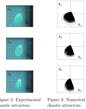
3 2 1 v v v 21 11 i 31 i i
1
0
0
全文
図
関連したドキュメント
Part V proves that the functor cat : glCW −→ Flow from the category of glob- ular CW-complexes to that of flows induces an equivalence of categories from the localization glCW[ SH −1
In the literature it is usually studied in one of several different contexts, for example in the game of Wythoff Nim, in connection with Beatty sequences and with so-called
Chaudhuri, “An EOQ model with ramp type demand rate, time dependent deterioration rate, unit production cost and shortages,” European Journal of Operational Research, vol..
In the first section we introduce the main notations and notions, set up the problem of weak solutions of the initial-boundary value problem for gen- eralized Navier-Stokes
At the same time we should notice that problems of wave propagation in a nonlinear layer that is located between two semi-infinite linear or/and nonlinear media are much more
By virtue of Theorems 4.10 and 5.1, we see under the conditions of Theorem 6.1 that the initial value problem (1.4) and the Volterra integral equation (1.2) are equivalent in the
On the other hand, modeling nonlinear dynamics and chaos, with its origins in physics and applied mathematics, usually concerned with autonomous systems, very often
iv Relation 2.13 shows that to lowest order in the perturbation, the group of energy basis matrix elements of any observable A corresponding to a fixed energy difference E m − E n
