A Series Solution of a Class of Diffusion Problems Arises During MRI
V. Soti
Department of Physics, Faculty of Sciences, Air University, Tehran, Iran.
Email: [email protected]
Abstract: In this study, the Diffusion Tensor Magnetic Resonance Imaging is investigated as a class of nonlinear diffusion equation subject to initial and boundary conditions. The Adomian Decomposition method is established for solving the proposed problem. The validity of this approach is investigate by using some numerical examples.
[V. Soti. A Series Solution of a Class of Diffusion Problems Arises During MRI. Academ Arena 2017;9(1):77- 81]. ISSN 1553-992X (print); ISSN 2158-771X (online). http://www.sciencepub.net/academia. 9.
doi:10.7537/marsaaj090117.09.
Keywords: MRI, Adomian decomposition method, diffusion equation.
1. Introduction
The recent introduction of DT-MRI (Diffusion Tensor Magnetic Resonance Imaging) has raised a strong interest in the medical imaging community.
Magnetic resonance imaging (MRI) uses the fact that under certain conditions the spin of hydrogen nuclei can be flipped from one state to another. By measuring the location of these flips, a picture can be formed of where the hydrogen atoms (mainly as a part of water) are in a body. magnetic resonance imaging (MRI) is based on effects that cross multiple biological levels: contrast depends on interactions between the local chemistry, water mobility, microscopic magnetic environment at the subcellular, cellular or vascular level, cellular integrity, etc. The success of diffusion MRI is deeply rooted in the powerful concept that during their random, diffusion- driven displacements molecules probe tissue structure at a microscopic scale well beyond the usual image resolution. The diffusion MRI can reveal orientation- dependent behavior of water molecules for localization of specific organs and pathologies, and for functionality assessment. As diffusion is truly a three dimensional process, molecular mobility in tissues may be anisotropic, as in brain white matter.
With diffusion tensor imaging (DTI), diffusion anisotropy effects can be fully extracted, characterized, and exploited, providing even more exquisite details on tissue microstructure. On the other hand, measuring diffusion in the real space, for instance water diffusion in a living body, is not a simple task though it provides useful and important information. Indeed, incoherent motion of water molecules has certain anisotropy in living bodies relating to normal and abnormal structures [1-5].
The “diffusion” may be one of the most important and attractive notions in mathematical methods for image analysis. Diffusion equation is one of the most important models which appears in the MRI, and often is nonlinear. Nonlinear partial
differential equations are encountered in such various fields as physics, mathematics and engineering. Most nonlinear models of real life problems are still very difficult to solve either numerically or theoretically.
There has recently been much attention devoted to the search for better and more efficient methods for determining a solution, approximate or exact, analytical or numerical, to the nonlinear models [1- 3,6-8,20].
2. Mathematical formulation
In this paper we consider a class of diffusion problems which arises in MRI frequently as follows:
t x x
u D x u x F u
x t T
=( ( ) ) ( ) ( ),
( , ) [0,1] [0, ] (1) 1
<
<
0 ), (
= ,0)
(x f x x
u , (2)
T t t
p t
u(0, )= ( ), 0< < , (3) T
t t
q t
ux(1, )= ( ), 0< <
, (4)
], [0, [0,1]
) , ( ,
|<
) , (
|u x t K x t T (5)
Where D x( )>0, (x),F(u), f(x), p(t) ,
and q(t) are known functions and K is a known constant. In addition we suppose that
) ( ), ( ),
(x f x p t
, and q(t) are point-wise
continuous functions, D(x)C1(0,1), and F(u)
is a continues Lipshits function; i.e. there exist a positive constant lR such that for each u1 and u2
.
|
|
| ) ( ) (
|F u1 F u2 l u1u2
(6)
In (1), D(x) represents the diffusive coefficient and (x)F(u) represents the source term. Here we represent an algorithm based on Adomian decomposition method (ADM) for solving the
problem (1)-(5). The ADM has been proved to be effective and reliable for handling differential equations, linear or nonlinear. Unlike the traditional methods, The ADM needs no discritization, linearization, spatial transformation or perturbation.
The ADM provide an analytical solution in the form of an infinite convergent power series. A large amount of research works has been devoted to the application of the ADM to a wide class of linear and nonlinear, ordinary or partial differential equations [7-13].
3. The base of Adomian decomposition method Let us first recall the basic principles of the ADM for solving differential equations. Consider the general equation: u= g , where represents a general nonlinear differential operator involving both linear and nonlinear terms. The linear term is decomposed into LR , where L is easily invertible and R is the remainder of the linear operator. For convenience, L may be taken as the highest order derivation. Thus the equation may be written as:
,
=q Nu Ru
Lu (7)
where Nu represents the nonlinear terms.
Solving Lu from (7), we have:
.
= g Ru Nu
Lu (8)
Since L is invertible, the equivalent expression is:
.
= 1 1 1
1Lu L g L Ru L Nu
L (9)
Therefor, u can be expressed as following series ,
=
0
= n n
u
u
(10)
with reasonable u0
which may be identified with respect to the definition of L1 and g , and
0
>
,n un
is to be determined. The nonlinear term Nu will be decomposed by the infinite series of Adomian polynomials
,
=
0
= n n
A Nu
(11)
where An
's are obtained by writing ,
= ) (
0
= n n n
u v
(12)
.
= )) ( (
0
= n n n
A v
N
(13)
Here is a parameter introduced for convenience. From (12) and (13), we have:
0.
, )]
(
! [
= 1 =0
0
=
u n d Nd
A n k k
k n n
n
(14)
The An
's are given as:
), (
= 0
0 F u
A
), (
= 0
0 1
1 F u
du u d A
), 2! (
) (
= 2 0
0 2 2 1 0 0 2
2 F u
du d u u
du F u d
A
A u d F u du
u
d d
u u F u F u
du du
3 3 0
0
3
2 3
1
1 2 2 0 3 0
0 0
= ( )
( ) ( ),
3!
Now, substituting (10) and (11) into (9) yields . )
(
=
0
= 1 0
= 1 0 0
=
n n n
n n
n
A L u R L u
u
(15) Consequently, with a suitable u0
we can write ,
= 1 0 1 0
1 L Ru L A
u
.
= 1 1
1 n n
n L Ru L A
u
All of un
are calculable, and u=
n=0un. Since the series converges and does so very rapidly, the n-term partial sum k
n k
n k u
s =
1=0can serve as a practical solution.
For the convergence of the decomposition method, the readers are referred to [13-19].
4. Method of solution
In this section, consider following linear operators
.
= ,
= ,
= 2
2
L t L x
Lxx x x t
(16)
Using this notation, the equation (1) becomes
).
( ) ( ) ) ( (
= )
(u L D x L u x F u
Lt x x
(17) By defining the inverse operators
1
Lt
one may formally obtain from (9) that
t x x
u x t f x
L L D x L u x F u
1
( , )= ( )
[ ( ( ) ) ( ) ( )],
(18)
where Lt (.)= t(.)d
0
1
. Now if we define
), (
= ) ,
0(x t f x
u (19)
we can seek the solution u(x,t) of the problem (1)-(5) based on Adomian decomposition approach as
).
, (
= ) , (
0
=
t x u t
x
u n
n
(20)
The nonlinear terms are decomposed as:
,
= ) (
0
= n n
A u
F
(21)
where An
, may be found as follows [5-8]
0.
, )]
(
! [
= 1 =0
0
=
n u
d F d
A n k k
k n n
n
(22)
Substituting (20) and (21) into (18) gives
n t x x n
n n
n n
u f x L L D x L u
x A
1
=0 =0
=0
= ( ) [ ( ( ) )
( ) ].
(23) Using above decomposition analysis, the following recurrence relation can be derived
) (
0 = f x
u , (24)
n
t x x n n
u
L L D x L u x A n
1 1
=
[ ( ( ) ) ( ) ], 0.
(25)
On the other hand, we may use the operator Lxx
and it's inverse to introduce the solution. Conditions (3) and (4) suggest defining the operator
1
Lxx
and the starting term as:
,
= 0 1
1 dx dx
Lxx
x
x (26)).
( ) (
= ) ,
0(x t p t xq t
u
(27)
Then the solution of problem (1)-(5) can be derived as follows:
n ,
n
u x t u x t
=0( , )= ( , )
(28)
where
n xx t n
x n n
u L L u
D x
D x L u x A n
1 1
= [ 1 {
( )
( ) ( ) }], 0.
(29) In (29), D x( ) shows the derivation of D(x)
with respect to variable x and the Adomian polynomial An
is obtained subject to un, n0
calculated using
1
Lxx
. The decomposition series (25) and (29) are generally convergent very rapidly in real physical problems. The convergence of the decomposition series have been investigated by several authors [5-8, 12, 13]. One can use each one of the decomposition series (25) or (29) for constructing the solution of the problem (1)-(5). In addition if one wants to introduce the solution with respect to the initial and boundary conditions (2)-(4), the average of the relations (25) or (29) can be used.
5. Numerical Experiments
In this section, for illustrations purpose we consider some problems and we show that how the ADM presented in the preceding section is computationally efficient.
Example 1.
Consider the following nonlinear diffusion problem
, ,
t xx
x
u u u u x t
u x sinx
u t u t
= (1 ), 0< < , 0< <1 3
( ,0)=
(0, )=0, ( , )=0.
(30) Using the recursive relation (25) yields
x u0 =sin
sin ,
t xx
u
u x A x d x t2 1= (0 0 ( , ) 0( , )) =
3
cos sin sin ,
t
u uxx x A x d
x x x t
2 0 1 1
2
2 2 3
= ( ( , ) ( , )) =
2 1
[( ( ) ]
3 9 2
sin ) 2 3(1 [8
= )) , ( ) , ( (
= 2 2 2
3 0 u x A x d x
u
t xx 3!, sin ] 27 sin 2
9 cos 1 3sin
sin 1 3
1 2 2 3 4 t3
x x
x x
x
and so on, the solution u(x, t) is in the following form:
).
, (
= ) , (
0
=
t x u t
x
u n
n
Example 2.
Consider following initial- boundary value problem
1 .
= 1 ) , ( 0,
= ) (0,
= ,0) (
1
<
<
0 ,
<
<
0 1 ,
=1 2
t t L u t
u
x x u
t L x xu
xu u
x xx
t
(31) Using the recursive relation (25) yields
x u0 =
,
= )) , ( ) , ( 1 (
= 0 0
1 0 u x A x d xt
u x
t xx 2 1
0 1
2 1 ( ( , ) ( , )) =
= u x A x d xt
u x
t xx 3 2
0 2
3 1 ( ( , ) ( , )) =
= u x A x d xt
u x
t xx 4 3
0 3
4 1 ( ( , ) ( , )) =
= u x A x d xt
u x
t xx and so on, the solution u(x, t) in a series form is given by
.
= ) , (
0
= n n
t x t x
u
Since 0<t<1, then we have
1 .
= ) ,
( t
t x x
u
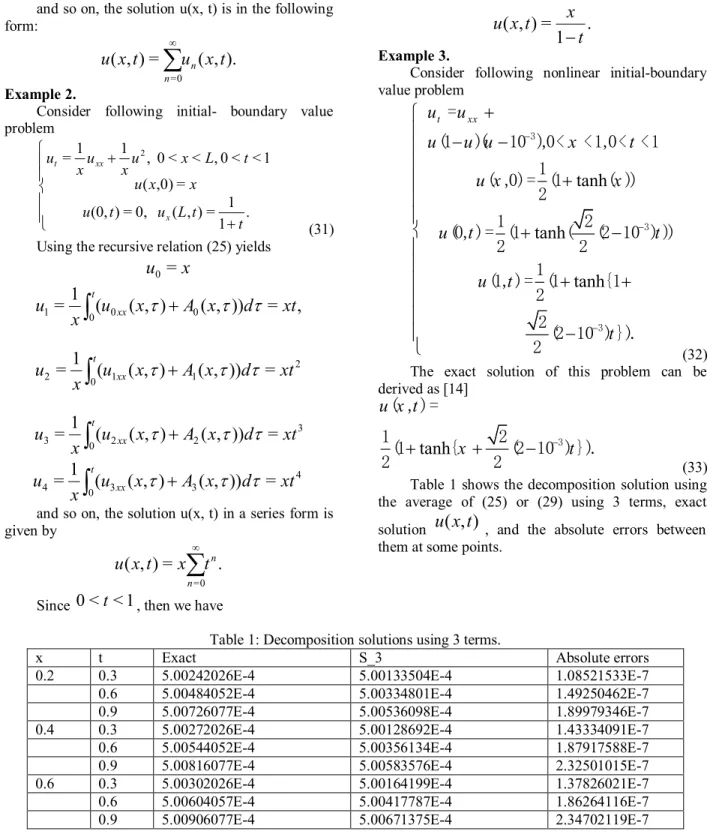
Example 3.
Consider following nonlinear initial-boundary value problem
tanh tanh
tanh
t xx
u u
u u u x t
u x x
u t t
u t
t
3
3
3
=
(1 )( 10 ),0< <1, 0< <1 ( ,0)= (11 ( ))
2
1 2
(0, )= (1 ( (2 10 ) ))
2 2
(1, )= (11 {1 2
2(2 10 ) }).
2 (32)
The exact solution of this problem can be derived as [14]
tanh u x t
x t
3
( , )=
1 2
(1 { (2 10 ) }).
2 2 (33)
Table 1 shows the decomposition solution using the average of (25) or (29) using 3 terms, exact solution u(x,t) , and the absolute errors between them at some points.
Table 1: Decomposition solutions using 3 terms.
x t Exact S_3 Absolute errors
0.2 0.3 5.00242026E-4 5.00133504E-4 1.08521533E-7
0.6 5.00484052E-4 5.00334801E-4 1.49250462E-7
0.9 5.00726077E-4 5.00536098E-4 1.89979346E-7
0.4 0.3 5.00272026E-4 5.00128692E-4 1.43334091E-7
0.6 5.00544052E-4 5.00356134E-4 1.87917588E-7
0.9 5.00816077E-4 5.00583576E-4 2.32501015E-7
0.6 0.3 5.00302026E-4 5.00164199E-4 1.37826021E-7
0.6 5.00604057E-4 5.00417787E-4 1.86264116E-7
0.9 5.00906077E-4 5.00671375E-4 2.34702119E-7
6. Conclusion
In this paper a class of diffusion equations subject to initial and boundary conditions is solved by using ADM. This class of problem appear during the modeling of a lot of physical phenomena specially in MRI. Using this method has this advantages that it needs no discritization, linearization, spatial
transformation or perturbation and it seems that ADM is a reasonable method for solving the nonlinear problems.
Corresponding Author:
V. Soti,
Department of Physics, Faculty of Sciences,
Air University, Tehran, Iran.
Email: [email protected] References:
1. Le Bihan D, Breton E. Imagerie de diffusion in vivo par re´sonance magne´tique nucle´aire. CR Acad Sci Paris 1985;301:1109–1112.
2. Merboldt KD, Hanicke W, Frahm J. Self- diffusion NMR imaging using stimulated echoes.
J Magn Reson 1985;64:479–486.
3. Taylor DG, Bushell MC. The spatial mapping of translational diffusion coefficients by the NMR imaging technique. Phys Med Biol 1985;30:345–
349.
4. Stejskal EO, Tanner JE. Spin diffusion measurements: spin echoes in the presence of a time-dependent field gradient. J Chem Phys 1965;42:288–292.
5. Le Bihan D, Breton E, Lallemand D, et al. MR imaging of intravoxel incoherent motions:
application to diffusion and perfusion in neurologic disorders. Radiology 1986;161:401–
407.
6. J.D. Logan, Nonlinear partial differential equations, Wiley/Interscience, New York, 1994.
7. A.Shidfar, M. Djalalvand, and M. Garshasbi, A numerical scheme for solving special class of nonlinear diffusion-convection equation, Appl.
Math. Copmut. 167 (2005) 1080-1089.
8. Shidfar, M. Garshasbi, A Weighted Algorithm Based on Adomian Decomposition Method for Solving an Special Class of Evolution Equations, Commun. Nonlinear Sci. Num. Simul. (in press).
9. D.Lesnic and L. Elliott, The decomposition approach to inverse heat conduction, J. Math.
Anal. Appl. 232 (1999) 82-98.
10. K. Abbaoui and Y. Cherruault, New ideas for proving convergence of decomposition method, Comput. Math. Appl. 29 (1995) 103-108.
11. G. Adomian, A review of the decomposition method and some recent results for nonlinear equation, Math. Comput. Model. 13 (1992) 7-17.
12. G. Adomian, Convergent series solution of nonlinear equations, J. Comput. Appl. Math. 2 (1984) 225-230.
13. G. Adomian, Solving frontier problems modelled by nonlinear partial differential equations, Comput. Math. Anal. 22 (1991) 91-94.
14. G. Adomian and R. Meyers, Nonlinear transport in moving fluids, Appl. Math. Lett. 6 (1993) 35- 38.
15. A.M. Wazwaz, A reliable modification of Adomian decomposition method, Appl. Math.
Comput. 175 (1999)77-86.
16. A.M. Wazwaz, S.M. EI-Sayed, A new modification of the Adomian decomposition method for linear and nonlinear operators, Appl.
Math. Comput. 122 (2001) 393-405.
17. D. Kaya and A. Yakus, A numerical comparison of partial solutions in the decomposition method for linear and nonlinear partial differential equations, Math. Comput. Simul. 60 (2002) 507- 512.
18. D. Kaya and I.E. Inan, A convergence analysis of the ADM and an application, Appl. Math.
Copmut. 161 (2005) 1015-1025.
19. A.D. polyanin and V.F. Zaistev, Handbook of nonlinear partial differential equations, Chapman Hall/CRC Press, Boca Raton, 2004.
1/25/2017