Experimental Study on Seismic Resistance of Indonesian Brick Masonry Houses

2016

Master’s Thesis

Experimental Study on Seismic Resistance of Indonesian Brick Masonry Houses

Adviser: Professor Toshikazu Hanazato

Department of Architecture, Graduate School of Engineering, Mie University

Yasuhide Senoo

Abstract

Indonesia has suffered severe damages by earthquakes. In particular, human casualty has mainly caused due to collapse of vulnerable brick masonry houses named non-engineered construction. These houses are built by local people who don’t have engineering skill and expertise. Therefore the major aim of this study is improvement of earthquake resistance for the typical brick masonry houses in Indonesia. The present paper describes dynamic seismic performance of Indonesian brick masonry houses with and without reinforcement and material characteristic. The reinforcement method was covering wire mesh which is available in local market and plaster mortar on both sides of walls. Shaking table test of full scale model

structure was conducted to clarify seismic performance and assess the effect of reinforcement.

Bricks were imported from Jakarta, Indonesia. Both of models survived without visible minor cracks until shaken by 675 gal. Upper west wall of non-reinforced model structure collapsed to out-of-plane direction shaken by 860 gal. On the other hand, reinforced model still survived without any cracks shaken by 2G. As a result of this shaking tests and comparison with past studies, reinforcement using ferrocement was effective to improve earthquake resistant strength of brick masonry structure and suppress deformation particularly out-of-plane wall.

Some of shaking table tests of full scale model structures revealed that the dynamic

deformability of brick masonry structure was roughly between 1/70 and 1/60 rad, both in-plane and out-of-plane. Natural frequency of out-of-plane vibration of masonry wall was obtained from response acceleration. Both models natural frequency became lower as shaking level was raised although there were no visible damages. It indicated that both models must have gotten invisible damages. The stiffness of non-reinforced wall reduced roughly 10%. It revealed that measuring free vibration of out-of-plane wall is possible to detect invisible damages.

Material strength test was conducted to reveal characteristic of local materials and calculate strength of model structures. Bending strength, rigidity, and natural frequency were obtained from the calculation. These results corresponded well with the shaking table test. These results showed that ferrocement layers strengthen bending strength roughly 5 times than original model.

Experimental Study on Seismic Resistance of

Indonesian Brick Masonry Houses

Contents

Chapter1. Introduction

1.1 Background ...1

1.2 Field Survey ...4

1.2.1 Outlines ...4

1.2.2 Brick Factory ...5

1.2.3 Construction site ...7

1.3 Past Studies ...12

Chapter2. Shaking table test of full scale model structure 2.1 Outlines ...15

2.2 Construction Process ...22

2.3 Measurement System ...24

2.3.1 Accelerometer ...24

2.3.2 3-D Image Processing ...25

2.4 Results ...28

2.4.1 Input Motion and Damage Description ...28

2.4.2 Response Acceleration ...32

2.4.3 Response Displacement ...40

2.4.4 Deformability ...55

(1)Out-Of-Plane (2)In-Plane (3)Comparison with Past Studies 2.4.5 Natural frequency of out-of-plane vibration of masonry wall ...64

2.4.6 Conclusions ...67

Chapter3. Material Tests 3.1 Brick size and density ...70

3.2 Compression Tests ...71

3.2.1 Brick ...71

3.2.2 Mortar ...72

3.2.3 Masonry Prism ...74

3.3 Tensile Tests ...72

3.3.1 Mortar ...75

3.3.2 Wire Mesh ...76

3.3.3 Ferrocement ...77

3.4 Bond Strength ...78

3.5 Shear strength ...79

3.6 Conclusions ...79

Chapter4. Quantitative Evaluation 4.1Earthquake resisting strength of model structures ...80

4.2 Simple Beam Model ...88

4.3 Conclusions ...90

Chapter5. Conclusions 5.1 Conclusion ...92

5.2 Further Studies ...93 Acknowledgements

0 200000 400000 600000 800000 1000000 India

Turkey Italy Pakistan Iran Islam Rep Soviet Union Japan Indonesia Haiti China

Number of deaths

Fig.1.1-2 Countries with the most earthquake fatalities 1900-2015^1-2)

Chapter1. Introduction

1.1 Background

Recent seismic activities that are increasing especially along Pan-Pacific zone is shown in Figure 1.1-1. It has caused serious damages in the disaster area. Figure 1.1-2 shows the ten countries with the most deaths resulting from earthquakes between 1900 and 2015. Total of number of deaths these countries, over 2 million people were killed by earthquakes.Earthquake disaster mitigation is an urgent issue for them.

Fig.1.1-1 Global Earthquakes 1900-2013^1-1)

It is noteworthy that Indonesia is the hardest-hit area in the past 14 years (See Table1.1-1, Fig.1.1-3). Approximately 2 hundred thousand people have died for past 115 years by earthquakes in this country (See Fig.1.1-2). This country has suffered from the largest earthquake and deadliest earthquake four times each from 1990 to 2014.

Year Data Magnitude Fatalities Region Year Data Magnitude Fatalities Region

2014 01-4 8.2 6

NW of Iquique, Chile

2014 03-8 6.2 729

near Wenping, China

2013 24-5 8.3 0 Sea of

Okhotsk 2013 24-9 7.7 825

61km NNE of Awaran, Pakistan/td>

2012 11-4 8.6 0

off the west coast of northern Sumatra

2012 06-2 6.7 113

Negros-Cebu region, Philippines

2011 11-3 9 20896

Near the East Coast of Honshu, Japan

2011 11-3 9 20896

Near the East Coast of Honshu, Japan

2010 27-2 8.8 507

Offshore Maule, Chile

2010 12-1 7 316000 Haiti

2009 29-9 8.1 192

Samoa Islands region

2009 30-9 7.5 1117

Southern Sumatra, Indonesia

2008 12-5 7.9 87587

Eastern Sichuan, China

2008 12-5 7.9 87587

Eastern Sichuan, China

2007 12-9 8.5 25

Southern Sumatera, Indonesia

2007 15-8 8 514

Near the Coast of Central Peru

2006 15-11 8.3 0 Kuril

Islands 2006 26-5 6.3 5749 Java,

Indonesia

2005 28-3 8.6 1313

Northern Sumatra, Indonesia

2005 08-10 7.6 80361 Pakistan

2004 26-12 9.1 227898

Off West Coast of Northern Sumatra

2004 26-12 9.1 227898

Off West Coast of Northern Sumatra

2003 25-9 8.3 0

Hokkaido, Japan Region

2003 26-12 6.6 31000 Southeastern

Iran

2002 03-11 7.9 0 Central

Alaska 2002 25-3 6.1 1000

Hindu Kush Region, Afghanistan

2001 23-6 8.4 138

Near Coast of Peru

2001 26-1 7.7 20023 India

2000 16-11 8 2

New Ireland Region, P.N.G.

2000 04-6 7.9 103

Southern Sumatera, Indonesia

Largest Earthquakes Deadliest Erathquakes

Table.1.1-1 Largest and Deadliest Earthquakes by year: 1990-2014^1-3)

Nearly 44,000 constructions got damages by the West Sumatra Earthquake, 2007.

Of these approximately 60% constructions, the damage appeared at medium and heavy level.

As a result, more than 135,000 people were displaced^1-4).

In 2 specific areas of Bandung state which were the worst –hit area by 2009 West Java Earthquake, over 76% all of buildings were residences and over 30% of this were

URM(Unreinforced masonry). These buildings sustained the most serious damage by the earthquake^1-5).

This kind of building is known as ‘non-engineered constructions’. They were not constructed by local people who did not have engineering skill and expertise, with poor local materials.

Whenever earthquake occurred, these buildings collapsed and got severe damage. It’s main cause of heavy casualties. For this reason, improvement of earthquake-resistant for non- engineered constructions is the most effective way to reduce interpersonal damage.

Fig.1.1-3 Seismicity map of Southeast Asia 1990-2012^1-1)

1.2 Field Survey 1.2.1 Outlines

On May 26, 2006, Mw 6.3 earthquake struck the island of Java. Over 5000 people were died by the earthquake. According to the damage reports^1-6), 154,000 houses were completely

destroyed, and 260,000 suffered some damage. In some villages, 70-90% of the houses were completely destroyed and URM were the most severely damaged. Bantul district in Yogyakarta Special Province has suffered the most severe damage due to the earthquake (See Fig.1.2-1, 2). 47,000 houses were destroyed in the area.

Field survey was conducted in Jogjakarta in end of November 2015. The main aim of this survey is to inspect a construction process of brick masonry houses and manufacturing process of the bricks. Some bricks and mortar samples were brought to Japan to conduct the mechanical tests of materials. Results of the survey are shown below.

Fig.1.2.1-1 Epicenter and damage map of 2006 Central Java Earthquake^1-7)

Fig.1.2.1-2 Destroyed Unreinforced Masonry Houses in Bantul^1-6)

1.2.2 Brick Factory

Brick manufacturing process in Kasongan, Bantul district in Jogjakarta is described below (See Fig.1.2.2-1). A worker is not only brick manufacturer, but also farmer mainly. Breaking ground with some water is a first step to make bricks. Soft clay containing water is molded into the form of rectangular solid. All of bricks are drawn curve as a signature before hardened. Molded clay is dried in the sun for 5 days and piled up. After that, it’s fired for 3 days. The main fuels are chaff and woods. There is no kiln in the factory. The fuel is filled to gap of piled bricks.

Some bricks were brought to Japan to conduct compressive strength test. The compressive strength of this brick was 4.2 N/mm² (See Table 1.2.2-1). Details of the specimen are shown in Fig.1.2.2-2 to 3.

①Breaking ground ②Molding clay into the rectangular solid

⑥After fired Fig.1.2.2-1 Brick manufacturing process (Kasongan, Bantul)

③Drawn a curve as a signature

④Dried in the sun

⑤Piled up before fired

D=3cm

H=3cm

Fig.1.2.2-2 Size of Kasongan Brick for Compressive test

Fig.1.2.2-3 Specimen of Kasongan Brick

1 2.2 4.7

2 2.2 4.7

3 2.1 4.4

4 2.1 4.4

5 1.9 2.9

6 2.0 4.0

Ave. 2.1 4.2

No. Compressive Strength (N/mm²)

Density (g/cm³)

Table 1.2.2-1 Compressive Strength of Brick made in Kasongan

1.2.3 Construction site

Fig.1.2.3-1 shows a single-story brick masonry house with RC frame under construction near the brick factory introduced in 1.2.2. Blending ratio of mortar of cement to sand is

approximately 1:5. Mixing mortar process is shown in Fig.1.2.3-3. Sand was filtered to remove impurities and make uniform grain size by wire mesh which has approximately 5 mm interval.

Filtered sand is mixed with cement and shaped like a volcano. Water is poured into the center of it and mixed with cement and sand on the ground. Compressive strength of this mortar was 2.3 N/mm² (See Table 1.2.3-1).

Fig.1.2.3-1 Exterior of brick masonry house under construction

Fig.1.2.3-2 Laying bricks

①Filtered sand and the detail of the wire mesh

②Poured water into sand and cement ③Water mixed with sand and cement Fig.1.2.3-3 Mixing mortar process

5cm

10cm

Fig.1.2.3-4 Size of mortar specimen for Compressive test

Fig.1.2.3-5 Mortar specimens for Compressive test

1 2.0 3.7

2 2.0 1.7

3 2.1 1.6

4 2.0 2.2

Ave. 2.0 2.3

No. Compressive Strength

(N/mm²) Density

(g/cm³)

Table 1.2.3-1 Compressive Strength of mortar

The width of joint mortar was 2cm to 3cm (See Fig.1.2.3-6). The interval of hoop tie bar was approximately 15cm and column main reinforcement consisted of round steel bars and deformed bars which the diameter was 10mm (See Fig.1.2.3-7).

Fig.1.2.3-8 shows a two-story brick masonry house with RC frame under construction in central Jogjakarta. Bamboos were used as timbering to support second floor temporarily. Bricks used for this house was made in Magelang, central Java (See Fig.1.2.3-9). The compressive strength of this brick was 10.5N/mm² (See Table 1.2.3-2). Compressive strength of this brick was over twice larger than bricks made in Kasongan.

Fig.1.2.3-6 Joint mortar and bricks Fig.1.2.3-7 Steal frame of RC column

Fig.1.2.3-8 Exterior of two-story brick masonry house under construction

Fig.1.2.3-9 Brick used for the house

3cm

3cm

Fig.1.2.3-10 Size of Megelang Brick for Compressive test

Fig.1.2.2-11 Specimen of Megelang Brick

1 2.28 13.4

2 2.32 11.5

3 2.20 8.38

4 2.19 9.04

5 2.23 8.75

6 2.20 9.81

7 2.31 12.9

8 2.27 10.5

Ave. 2.25 10.5

No. Compressive Strength (N/mm²)

Density (g/cm³)

Table 1.2.3-2 Compressive Strength of Brick made in Magelang

Column main reinforcements were bent so that it can be brought the construction site and straighten with hands (See Fig.1.2.3-12, 13). Columns are assembled after hoop ties made (See Fig.1.2.3-14, 15).

Fig.1.2.3-12 Bent column main reinforcements Fig.1.2.3-13 Making iron bar straighter

Fig.1.2.3-14 Making hoop ties Fig.1.2.3-15 Assembling the column

1.3 Past Studies

Through the past experiences and studies, weak points of brick masonry buildings have revealed. Fig.1.3-1 shows typical damage of non-engineered constructions^1-8)

A.Nakatani conducted shaking table test of full scale model structure in order to investigate the seismic behavior of Indonesian brick masonry house with the retrofitting reinforcement. The model structure had walls with and without wire mesh although all of walls were covered by mortar. Figure 1.3-2 shows the detail of retrofit reinforcement on the model. South wall which was without wire mesh cracked from the corner of window frame firstly and it triggered to collapse half part of south wall and whole east wall although walls with wire mesh withstood the shaking. The result revealed that seismic reinforcement using ferrocement is effective to prevent collapse^{1-9, 10)}.

K. Kobayashi carried out 3 types of full scale shaking table tests for Asian brick masonry houses. The first one was South Asian type of masonry house constructed by bricks imported from Pakistan. This model was laid by English bond because of common way in the area. The second one was South-East Asian type of confined masonry house which had RC frame. This model was designed based on Indonesian confined masonry houses although north wall was made by Japanese bricks. The third one was constructed by Peruvian bricks and had RC lintel beam for seismic reinforcement. These experiments revealed that seismic performance depends to a larger extent on strength of each materials and construction condition1-11, 12, 13). Some other seismic reinforcement methods are now under study. T. Narafu et al. proposed seismic base isolation sliding device using stones. Advantages of using stone are that it’s

Fig.1.3-1 Typical damage of non-engineered constructions^1-8)

・Wall: 3600×2600(mm)

・Brick: 210×100×50(mm)

・Finishing Mortar & Bond Mortar:

Cement: sand=1:6

Fig.1.3-2 Outline of model structure for previous shaking table experiment in 2012^1-9) higher durable than rubber and gathering materials easily^1-14). T. Sakurai supposed a method using PET-band. This band is used for heavy packing in large area^1-15).

With the points above considered, the aim of this study is to propose more effective seismic reinforced model using ferrocement, and investigate seismic performance by full scale shaking test. Additionally, quantitative evaluating the effect of seismic reinforcement based on the experiments is also purpose of this study.

References

1-1) USGS :http://www.usgs.gov/

1-2) Statista:http://www.statista.com/statistics/269649/earthquake-deaths-by-country/

1-3) USGS:http://earthquake.usgs.gov/earthquakes/eqarchives/year/byyear.php) 1-4) Miyamoto: 2007 West Sumatra Earthquake Reconnaissance Report, Miyamoto International, USA. 2007

1-5) Choi Ho et al., Report on Building Damage Investigation of the 2009 West Java Earthquake, Indonesia, Part1. Damage Overview and Damage Ratio Evaluation of Specific Area, AIJ, Aug. 2010

1-6) The Mw 6.3 Java, Indonesia, Earthquake of May 27, 2006, EERI Special Earthquake Report, August 2006

1-7) Pacific Disaster Management Information Network (PDMIN) http://photos1.blogger.com/blogger/8175/41/1600/image002.jpg

1-8) Teddy Boen, Published by UNCRD, Retrofitting Simple Buildings Damaged by Earthquakes, 2010

1-9) A. Nakatani, Experimental study for mitigation of earthquake disaster of ordinary masonry houses in developing countries, Master’s thesis, Dept. Arch., Mie University, 2013

1-10) Teddy Boen et al., Brief Report of Shaking Table Test on Masonry Building Strengthened with Ferrocement Layers, Journal of Disaster Research Vol. 10 No.3, 2015

1-11) K. Kobayashi, 途上国のレンガ組積造住宅の耐震性に関する実験研究 (Experimental study for seismic performance of brick masonry houses in developing countries), Dept. of Arch, Grad. School of Eng. Mie University, 2009

1-12) K. Kobayashi et al., Study about Seismic Construction of Masonry Housing in Developing Country Part.2 Shaking table test of model structure of brick house, AIJ 2008

1-13) H. Imai et al., Experimental Study on Confined Masonry Structure for Earthquake Safety Design –Full scale shaking table test and cyclic loading test-, AIJ J. Technol. Des.

Vol.16, No.32, 151-156, Feb, 2010

1-14) N. Yamaguchi et al., Development of simple and affordable seismic base isolation sliding device using stones, AIJ , pp423-424, 2008

1-15) T. Sakurai, Evaluation of the Effects of Seismic Retrofit for Masonry Structures using PET-band, Report of Graduate School, Dept. Engineering, Chuo University, 2013

Chapter2. Shaking table tests of full scale model structure

2.1 Outline

Full scale shaking table test was conducted to investigate the seismic performance of

Indonesian brick masonry houses. This experiment was conducted as collaborative research with NIED and Mie University from 4th to 5th June, 2014. The major aim of this experiment is to assess effectiveness of seismic reinforcement using ferrocement. Model A was typical Indonesian unreinforced masonry house, and Model B was same masonry structure

strengthened partially by ferrocement layers on both side of the walls, as sandwich structure.

This reinforced model was planned based on the guidebook^1-8). Bricks and wire mesh with 2.5

×2.5cm rectangular grid used for reinforcement were imported from Jakarta, Indonesia.

Blending ratio of joint mortar of cement to sand was 1:6 by volume and water to cement was 120 % by weight. These ratios were based on common practice in the area. On the other hand, blending ratio of mortar used for reinforcement of cement to sand was 1:4 by volume and water to cement was 67% by weight. Details of model structures are shown in Fig.2.1-1 to 2.1-5.

Specification of the shaking table and plan of large-scale Earthquake simulator in NIED are shown in Fig.2.1-6 and Table 2.1-1.

Model A: Non-reinforced model Brick: made in Indonesia Joint mortar: cement 1: sand 6

Model B: Reinforced model Brick: made in Indonesia Joint mortar: cement 1: sand 6 Reinforced by wire mesh and mortar cement 1: sand 4

3700

3700 2600

(mm)

Shaking Direction

Fig.2.1-1Model Structures

wire mesh: Φ1mm@25mm

100 20 20

100 (mm)

East South

West North

Fig.2.1-2 Elevations of Model A

3700 3700

(A) North Elevation (B) South Elevation

(D) East Elevation (C) West Elevation

Fig.2.1-3 Elevations of Model B^2-1)

Fig.2.1-4 Arrangement of wire mesh on Model B^2-1)

500500 500

500

500 500

500 Retrofitting: Wire mesh, Galvanized welded iron, 25 mm grid 1mm diameter.

Finishing Mortar:

Cement:Sand=1:4

Hole & wire to stitch the inside-outside of wiremesh

Fix to Concrete foundation by concrete nail Countiguous wire mesh

(width 1000 mm) should be used

Countiguous wire mesh (width 1000 mm) should be used

Fig.2.1-5 Detail of installing wire mesh on Model B^2-1)

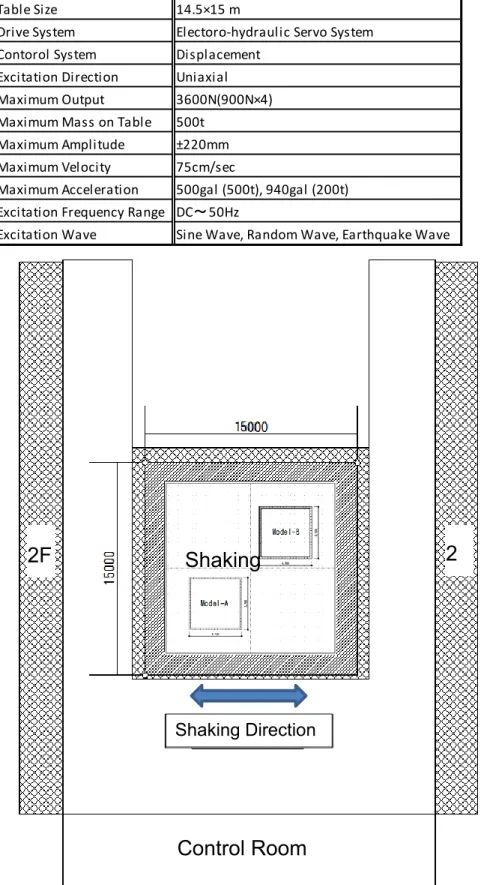
Table Size 14.5×15 m

Drive System Electoro-hydraulic Servo System Contorol System Displacement

Excitation Direction Uniaxial Maximum Output 3600N(900N×4) Maximum Mass on Table 500t

Maximum Amplitude ±220mm Maximum Velocity 75cm/sec

Maximum Acceleration 500gal (500t), 940gal (200t) Excitation Frequency Range DC～50Hz

Excitation Wave Sine Wave, Random Wave, Earthquake Wave Table 2.1-1 Specification of the shaking table

2F 2

Shaking F Table

Shaking Direction

Control Room (2F)

Fig. 2.1-6 Plan of Large-scale Earthquake Simulator in NIED

2.2 Construction Process

Both of models were constructed by local materials. Bricks were imported from Jakarta, Indonesia and wire mesh used for reinforcement was sold in local market (See Fig.2.2-1). The size of bricks is approximately L:200×W:100×T:50(mm). Grid space of the wire mesh is 2.5 cm and the diameter is 1 mm. Bricks were soaked to prevent absorb water from mortar (See Fig.2.2-2).

After soaking, bricks were laid by stretcher bond up to 2.6 m in height of south, north walls and 3.7 m totally in height of east, west walls (See Fig.2.2-3). Roofing nails were inserted in joint mortar of Model B before hardening to keep space 1cm between mortar face and wire mesh.

Binding wires were also inserted in joint mortar spaced 20cm to stitch wire mesh both inside and outside (See Fig.2.2-4).

Fig. 2.2-1 Indonesian bricks from Jakarta Fig. 2.2-2 Soaked bricks

Fig. 2.2-3 Model brick masonry houses

under construction Fig. 2.2-4 Inserted roofing nails and bending wire

After those working, walls are covered by wire mesh and tied with bending wire to connect both sides (See Fig.2.2-5). Mortar was spread on the wire mesh 2cm in thickness finally (See Fig.2.2-6). Fig.2.2-7 shows the detail and cross section of reinforced wall.

Fig. 2.2-5 Walls covered by wire mesh Fig. 2.2-6 Spreading mortar on wire mesh

Fig.2.2-7 Details of retrofitting with wire mesh covered by mortar^1-8)

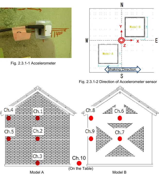
Fig. 2.3.1-1 Accelerometer

Shaking Direction

Fig. 2.3.1-2 Direction of Accelerometer sensor Z X

ｘ Y

2.3 Measurement System 2.3.1 Accelerometer

10 accelerometers in total were installed on east wall of both models and shaking table. All of accelerometers measure X-axis direction (See Fig. 2.3.1-2). The measurement point is shown in Fig.2.3.1-3.

Model A Model B

Ch.10

(On the Table) Fig. 2.3.1-3 Position of accelerometers

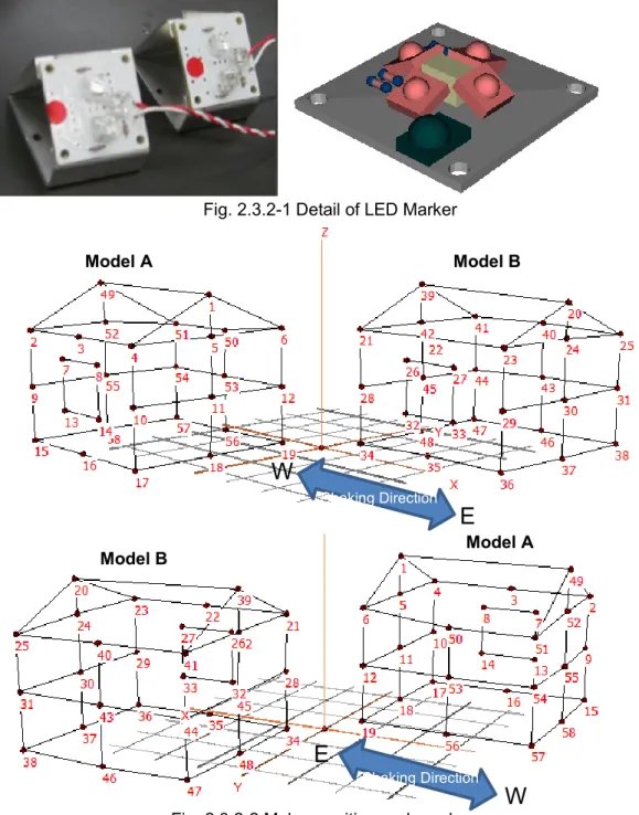
2.3.2 3-D image processing

Dynamic deformation was measured by 3-D image processing using LED markers in

cooperation with Prof. Niitsu, Tokyo Denki University. The size of the marker is W30, D30, H10 (mm) and weight is 5g (See Fig. 2.3.2-1). 29 Markers were installed in each model by double- sided adhesive tape. Maker position and number are shown in Fig.2.3.2-2 and Table 2.3.2-1.

The high speed cameras can record 100 times per second. Camera position is shown in Fig.

2.3.2-3 and Table 2.3.2-2. East direction, North direction and vertical direction are positive of X, Y, Z-axis respectively. The original is at the center of the models. (See Fig.2.2.3-2)

Model A Model B

Shaking Direction

W

E

Model B Model A

Shaking Direction

W E

Fig. 2.3.2-2 Maker position and number Fig. 2.3.2-1 Detail of LED Marker

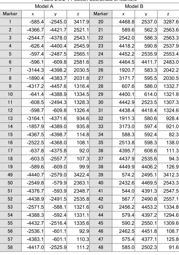
Table 2.3.2-1 Position Coordinate of Markers

Model A Model B

Marker x y z Marker x y z

1 -585.4 -2545.0 3417.9 20 4468.8 2537.0 3287.6 2 -4366.7 -4421.7 2521.1 21 589.6 562.3 2563.6 3 -2544.7 -4378.0 2543.1 22 2542.0 586.3 2563.3 4 -626.4 -4400.4 2545.9 23 4418.2 590.8 2537.9 5 -597.4 -2487.5 2565.1 24 4452.2 2535.9 2553.4 6 -596.1 -609.8 2581.6 25 4464.5 4411.7 2483.0 7 -3144.3 -4398.2 2030.5 26 1920.7 583.3 2042.2 8 -1890.4 -4383.7 2031.8 27 3171.7 595.5 2030.5 9 -4317.2 -4457.6 1316.4 28 607.6 586.0 1332.7 10 -641.4 -4388.9 1334.5 29 4400.1 614.0 1321.8 11 -608.5 -2494.3 1328.3 30 4442.9 2523.5 1307.3 12 -598.7 -609.8 1326.4 31 4438.4 4418.4 1324.6 13 -3164.1 -4371.6 934.6 32 1911.3 580.6 928.4 14 -1857.9 -4389.0 935.8 33 3173.0 597.4 921.0 15 -4367.5 -4398.7 114.8 34 588.3 592.4 82.3 16 -2522.5 -4368.0 108.1 35 2513.8 598.3 138.0 17 -637.8 -4375.8 92.0 36 4395.7 608.6 111.3 18 -603.5 -2557.7 107.3 37 4437.9 2535.6 94.3 19 -589.6 -609.0 99.9 38 4449.9 4406.2 126.9 49 -4440.7 -2579.0 3422.4 39 574.2 2495.1 3412.3 50 -2549.8 -579.9 2363.1 40 2432.6 4469.5 2543.3 51 -4376.7 -593.9 2348.7 41 544.0 4391.3 2547.5 52 -4438.9 -2491.5 2535.8 42 567.7 2490.8 2557.1 53 -2571.5 -588.1 1321.6 43 2456.2 4453.2 1334.8 54 -4388.3 -592.4 1331.1 44 579.4 4397.2 1294.6 55 -4432.7 -2516.4 1335.6 45 590.2 2550.1 1309.6 56 -2536.1 -601.1 92.9 46 2462.5 4451.8 108.7 57 -4383.1 -601.1 110.3 47 575.4 4377.1 125.8 58 -4417.0 -2525.9 111.2 48 585.0 2502.3 91.6

Camera No. x y z

1 6410 -11782 1825

2 10014 -10045 1353

3 -10905 8070 1996

4 -7844 11761 2579

Table 2.3.2-2 Camera Position

Fig. 2.3.2-3 Model structures and camera position Camera 1

Camera 2 Camera 3

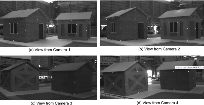
Camera 4

(a) View from Camera 1 (b) View from Camera 2

(c) View from Camera 3 (d) View from Camera 4

Fig. 2.3.2-4 View from High Speed Cameras

Calculation procedure of 3-D image is shown as below.

1) Measuring initial position of LED markers using 3-D measuring instrument, Set330RS.

2) Setting up high speed cameras and storing data

3) 3-D coordinates of marker positions were calculated by image data.

4) Obtaining relative displacement from shaking table and initial marker position based on above process.

2.4 Results

2.4.1 Input Motion and Damage Description

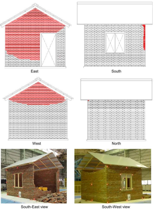
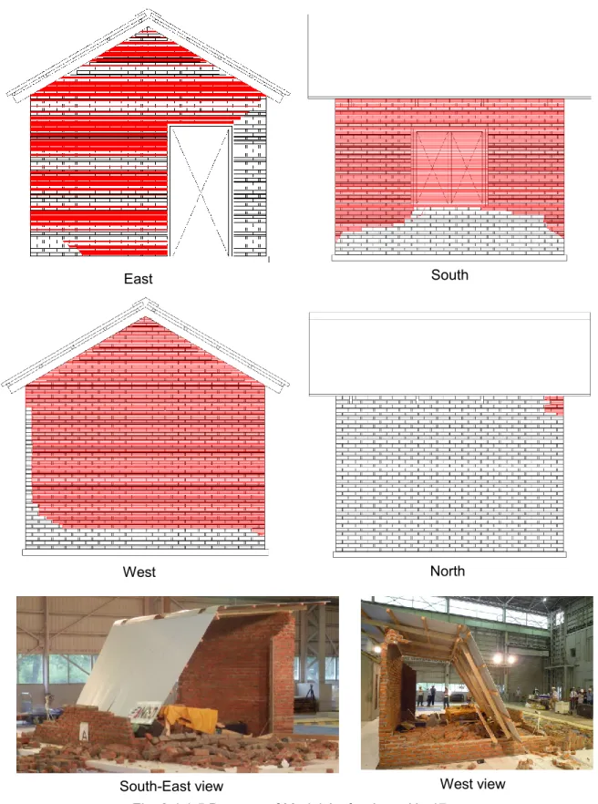
Excitation schedule of the shaking test and detail of structure damage are shown in Table 2.4.1-1. Input waves were based on The Southern Hyogo prefecture earthquake in 1995 and the excitation scale was based on amplitude ratio (See Fig.2.4.1-1, 2). Step waves were inputted after each excitation of JMA Kobe NS wave to know natural frequency (See Fig. 2.4.1- 3). Damages of the structures were observed by sight and recorded after each step wave inputted. Both of models didn’t get any visible damages until excitation No.12. Model A suffered severe damage due to excitation No. 13. Whole east wall and upper part of west wall collapsed by out-of-plane loading (See Fig.2.4.1-4). On the other hand, Model B still didn’t suffer any damages. Both models were shaken by 2.7G at last. Model A was completely

destroyed due to the excitation. Rest part of west wall collapsed first and immediately after that, south wall collapsed (See Fig. 2.4.1-5). Finally Model B didn’t suffer any damages (See Fig.

2.4.1-6).

Model A Model B

1 Step 1 - 0.5 -

2 JMA Kobe NS_20% 1 35 172

3 Step 2 - 0.5 -

4 JMA Kobe NS_35% 1 61 292

5 Step 3 - 0.5 -

6 JMA Kobe NS_50% 1 88 398

7 Step 4 - 0.5 -

8 JMA Kobe NS_60% 1 105 469

9 Step 5 - 0.5 -

10 Step 6 - 0.5 -

11 JMA Kobe NS_85% 1 149 675

12 Step 7 - 0.5 -

13 JMA Kobe NS_100% 1 175 860

Upper part of west wall and whole east wall collapsed [Fig.2.4.1-4]

14 Step 8 - 0.5 -

15 JMA Kobe NS_110% 1 193 1086

16 Step 9 - 0.5 -

17 JMA Kobe NS_100% 0.5 87.5 2607

All of walls collapsed completely except for north wall [Fig.2.4.1-5]

18 Step 10 - 0.5 - Unchanged

Time Scale

4th June, 20145th June, 2014

Date No. Input Wave

Unchanged

No damage Amplitude

(mm)

Acceleration (gal)

Damage

No damage Table 2.4.1-1 Excitation schedule and damage

-1000 -500 0 500 1000

0 10 20 30 40 50 60 70 80 90 100

Acceleratio (gal)

time (s)

Fig.2.4.1-1 No.13 Input Wave

-2800 -2100 -1400 -700 0 700 1400 2100 2800

0 5 10 15 20 25 30 35 40 45 50

Acceleration (gal)

time (s)

Fig.2.4.1-2 No.17 Input Wave

-200 -100 0 100 200

0 5 10 15 20 25 30 35 40

Acceleration (gal)

time (s) Fig.2.4.1-3 No.1 Input Wave

East

West North

South

South-West view South-East view

Fig. 2.4.1-4 Damage of Model A after Input No.13

Fig. 2.4.1-5 Damage of Model A after Input No.17 East

West

South

North

South-East view West view

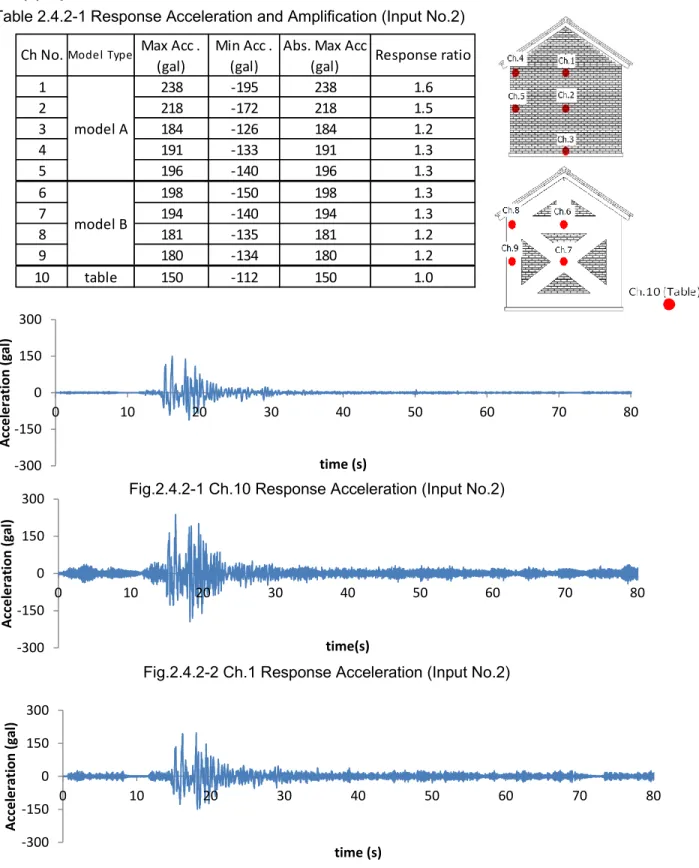
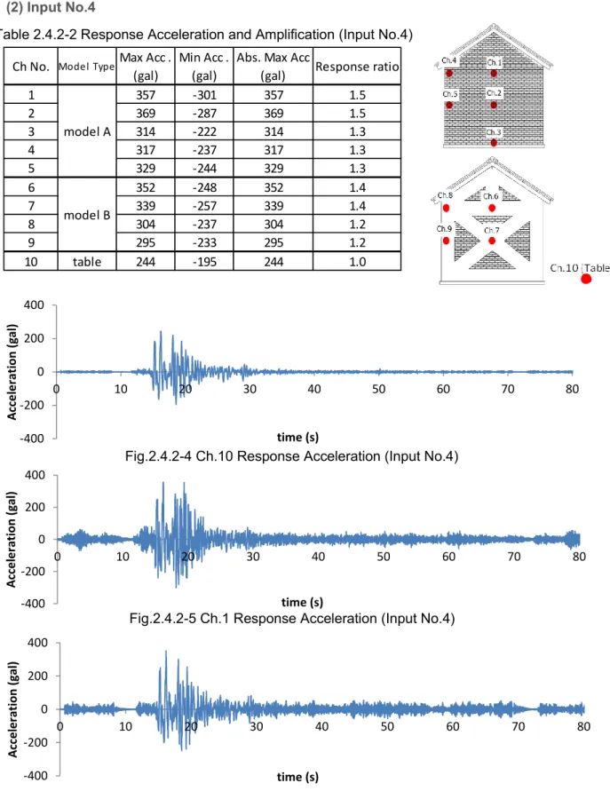
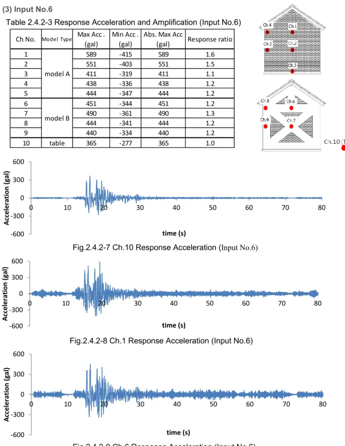
2.4.2 Response Acceleration

Out-of-plane response accelerations are given as below. Response ratio is based on response acceleration recorded by Ch.10 which was installed on shaking table. Behavior of Model A was recorded until excitation No.11 because the model collapsed next excitation with accelerometers. All of accelerometers were removed from both models before the last excitation. The maximum response acceleration ratio of Model A was 1.7 on Ch.1 (See 2.4.2-(5)). On the other hand, the maximum response acceleration ratio of Model B was 1.3 on Ch.7 (See 2.4.2-(7)).

South-East view

North-West view

Fig.2.4.1-6 Both Models after Input No.17

(1) Input No.2

-300 -150 0 150 300

0 10 20 30 40 50 60 70 80

Acceleration (gal)

time (s)

Fig.2.4.2-1 Ch.10 Response Acceleration (Input No.2)

-300 -150 0 150 300

0 10 20 30 40 50 60 70 80

Acceleration (gal)

time(s)

Fig.2.4.2-2 Ch.1 Response Acceleration (Input No.2)

-300 -150 0 150 300

0 10 20 30 40 50 60 70 80

Acceleration (gal)

time (s)

Fig.2.4.2-3 Ch.6 Response Acceleration (Input No.2)

1 238 -195 238 1.6

2 218 -172 218 1.5

3 184 -126 184 1.2

4 191 -133 191 1.3

5 196 -140 196 1.3

6 198 -150 198 1.3

7 194 -140 194 1.3

8 181 -135 181 1.2

9 180 -134 180 1.2

10 table 150 -112 150 1.0

Response ratio

model A

model B

Model Type

Ch No. Max Acc . (gal)

Min Acc . (gal)

Abs. Max Acc (gal)

Table 2.4.2-1 Response Acceleration and Amplification (Input No.2)

(2) Input No.4

1 357 -301 357 1.5

2 369 -287 369 1.5

3 314 -222 314 1.3

4 317 -237 317 1.3

5 329 -244 329 1.3

6 352 -248 352 1.4

7 339 -257 339 1.4

8 304 -237 304 1.2

9 295 -233 295 1.2

10 table 244 -195 244 1.0

Response ratio

model A

model B

Ch No. Model TypeMax Acc . (gal)

Min Acc . (gal)

Abs. Max Acc (gal)

Table 2.4.2-2 Response Acceleration and Amplification (Input No.4)

-400 -200 0 200 400

0 10 20 30 40 50 60 70 80

Acceleration (gal)

time (s)

Fig.2.4.2-4 Ch.10 Response Acceleration (Input No.4)

-400 -200 0 200 400

0 10 20 30 40 50 60 70 80

Acceleration (gal)

time (s)

Fig.2.4.2-5 Ch.1 Response Acceleration (Input No.4)

-400 -200 0 200 400

0 10 20 30 40 50 60 70 80

Acceleration (gal)

time (s)

Fig.2.4.2-6 Ch.6 Response Acceleration (Input No.4)

(3) Input No.6

1 589 -415 589 1.6

2 551 -403 551 1.5

3 411 -319 411 1.1

4 438 -336 438 1.2

5 444 -347 444 1.2

6 451 -344 451 1.2

7 490 -361 490 1.3

8 444 -341 444 1.2

9 440 -334 440 1.2

10 table 365 -277 365 1.0

Response ratio

model A

model B

Ch No. Model Type Max Acc . (gal)

Min Acc . (gal)

Abs. Max Acc (gal)

Table 2.4.2-3 Response Acceleration and Amplification (Input No.6)

-600 -300 0 300 600

0 10 20 30 40 50 60 70 80

Acceleration (gal)

time (s)

Fig.2.4.2-7 Ch.10 Response Acceleration (Input No.6)

-600 -300 0 300 600

0 10 20 30 40 50 60 70 80

Acceleration (gal)

time (s)

Fig.2.4.2-8 Ch.1 Response Acceleration (Input No.6)

-600 -300 0 300 600

0 10 20 30 40 50 60 70 80

Acceleration (gal)

time (s)

Fig.2.4.2-9 Ch.6 Response Acceleration (Input No.6)

(4) Input No.8

1 684 -613 684 1.6

2 631 -554 631 1.5

3 491 -388 491 1.2

4 523 -419 523 1.2

5 530 -417 530 1.2

6 533 -412 533 1.3

7 562 -430 562 1.3

8 533 -415 533 1.3

9 519 -408 519 1.2

10 table 425 -340 425 1.0

Response ratio

model A

model B

Ch No. Model Type Max Acc . (gal)

Min Acc . (gal)

Abs. Max Acc (gal)

Table 2.4.2-4 Response Acceleration and Amplification (Input No.8)

-800 -400 0 400 800

0 10 20 30 40 50 60 70 80

Acceleration (gal)

time (s)

Fig.2.4.2-10 Ch.10 Response Acceleration (Input No.8)

-800 -400 0 400 800

0 10 20 30 40 50 60 70 80

Acceleration (gal)

time (s)

Fig.2.4.2-11 Ch.1 Response Acceleration (Input No.8)

-800 -400 0 400 800

0 10 20 30 40 50 60 70 80

Acceleration (gal)

time (s)

Fig.2.4.2-12 Ch.6 Response Acceleration (Input No.8)

(5) Input No.11

1 889 -1017 1017 1.7

2 807 -770 807 1.4

3 721 -623 721 1.2

4 738 -657 738 1.2

5 755 -669 755 1.3

6 788 -662 788 1.3

7 828 -699 828 1.4

8 736 -651 736 1.2

9 721 -636 721 1.2

10 table 597 -524 597 1.0

Response ratio

model A

model B

Ch No. Model Type Max Acc . (gal)

Min Acc . (gal)

Abs. Max Acc (gal)

Table 2.4.2-5 Response Acceleration and Amplification (Input No.11)

-1200 -600 0 600 1200

0 10 20 30 40 50 60 70 80

Acceleration (gal)

time (s)

Fig.2.4.2-13 Ch.10 Response Acceleration (Input No.11)

-1200 -600 0 600 1200

0 10 20 30 40 50 60 70 80

Acceleration (gal)

time (s)

Fig.2.4.2-14 Ch.1 Response Acceleration (Input No.11)

-1200 -600 0 600 1200

0 10 20 30 40 50 60 70 80

Acceleration (gal)

time (s)

Fig.2.4.2-15 Ch.6 Response Acceleration (Input No.11)

(6) Input No.13

6 957 -797 957 1.2

7 1027 -846 1027 1.3

8 944 -805 944 1.2

9 922 -783 922 1.2

10 table 769 -640 769 1.0

Abs. Max Acc

(gal) Response ratio

model B

Ch No. Model Type Max Acc . (gal)

Min Acc . (gal)

Table 2.4.2-6 Response Acceleration and Amplification (Input No.13)

-1000 -500 0 500 1000

0 10 20 30 40 50 60 70 80

Acceleration (gal)

time (s)

Fig.2.4.2-16 Ch.10 Response Acceleration (Input No.13)

-1000 -500 0 500 1000

0 10 20 30 40 50 60 70 80

Acceleration (gal)

time (s)

Fig.2.4.2-17 Ch.6 Response Acceleration (Input No.13)

(7) Input No.15

6 1211 -944 1211 1.2

7 1294 -989 1294 1.3

8 1242 -947 1242 1.2

9 1207 -924 1207 1.2

10 table 995 -753 995 1.0

Response ratio

model B

Ch No. Model Type Max Acc . (gal)

Min Acc . (gal)

Abs. Max Acc (gal)

Table 2.4.2-7 Response Acceleration and Amplification (Input No.15)

-1400 -700 0 700 1400

0 10 20 30 40 50 60 70 80

Acceleration (gal)

time (s)

Fig.2.4.2-18 Ch.10 Response Acceleration (Input No.15)

-1400 -700 0 700 1400

0 10 20 30 40 50 60 70 80

Acceleration (gal)

time (s)

Fig.2.4.2-19 Ch.6 Response Acceleration (Input No.15)

2.4.3 Response Displacement

Response displacements were recorded by 3D image processing. Maximum response displacements by each excitation are shown in Table.2.4.3-1 to 7. These displacements are relative between each markers and M36. Maximum relative displacement of Model A to out-of- plane direction was 26.7 mm by excitation No.11 which was recorded by Ch.49 installed at top of the west wall (See Table.2.4.3-5). On the other hand, M39 installed top of the west wall of Model B recorded 8.9 mm by excitation No.15 (See Table 2.4.3-7). Top of the west wall of Model A displaced approximately 3 times larger than same point of Model B to out-of-plane direction.

Fig.2.4.3-25 shows the transition of out-of-plane displacement (negative direction of the X axis).

About Model B, relationship between input acceleration and response displacement is approximated by a straight line. On the other hand, displacement of Model A increased exponentially by excitation No.11 and displacement increased non-liner.

(1) Input No.2

Disp.

(Max)

Disp.

(Min)

Max.Disp.

(Abs. Value)

Residual Disp

X(mm) Y(mm) Z(mm) mm mm mm mm

1 -585.4 -2545 3417.9 X 5.57 -2.36 5.57 0.24

2 -4366.7 -4421.7 2521.1 X 2.81 -5.87 5.87 -3.38

3 -2544.7 -4378 2543.1 X 3.01 -3.83 3.83 -1.44

4 -626.4 -4400.4 2545.9 X 3.96 -2.76 3.96 0.81

5 -597.4 -2487.5 2565.1 X 4.68 -3.1 4.68 1.6

6 -596.1 -609.8 2581.6 X 6.86 -1.54 6.86 3.71

7 -3144.3 -4398.2 2030.5 X 4.93 -1.08 4.93 1.67

8 -1890.4 -4383.7 2031.8 X 2.88 -3.21 3.21 -1.22

9 -4317.2 -4457.6 1316.4 X 2.24 -4.17 4.17 -1.92

10 -641.4 -4388.9 1334.5 X 3.59 -1.76 3.59 0.15

11 -608.5 -2494.3 1328.3 X 5.62 -2.06 5.62 -0.45

12 -598.7 -609.8 1326.4 X 3.94 -3.03 3.94 0.42

13 -3164.1 -4371.6 934.6 X 2.36 -2.99 2.99 -0.94

14 -1857.9 -4389 935.8 X 3.14 -3.39 3.39 -1.74

15 -4367.5 -4398.7 114.8 X 4.93 -2.74 4.93 1.97

16 -2522.5 -4368 108.1 X 4.68 -2.24 4.68 1.64

17 -637.8 -4375.8 92 X 7.2 -2.68 7.2 1.6

18 -603.5 -2557.7 107.3 X 3.73 -2.63 3.73 1.35

19 -589.6 -609 99.9 X 8.24 -10.84 10.84 3.48

49 -4440.7 -2579 3422.4 X 3.57 -2.09 3.57 1.41

50 -2549.8 -579.9 2363.1 X 2.53 -3.24 3.24 0.8

51 -4376.7 -593.9 2348.7 X 1.65 -2.27 2.27 -1.21

52 -4438.9 -2491.5 2535.8 X 3.66 -2.08 3.66 -0.94

53 -2571.5 -588.1 1321.6 X 2.78 -2.37 2.78 0.83

54 -4388.3 -592.4 1331.1 X 3.02 -1.91 3.02 0.08

55 -4432.7 -2516.4 1335.6 X 2.65 -1.87 2.65 1.17

56 -2536.1 -601.1 92.9 X 2.83 -1.74 2.83 0.59

57 -4383.1 -601.1 110.3 X 2.72 -1.94 2.72 0.24

58 -4417 -2525.9 111.2 X 2.77 -1.53 2.77 1.19

20 4468.8 2537 3287.6 X 4.71 -1.53 4.71 2.93

21 589.6 562.3 2563.6 X 3.22 -2.5 3.22 0.74

22 2542 586.3 2563.3 X 3.04 -2.21 3.04 0.29

23 4418.2 590.8 2537.9 X 1.48 -1.77 1.77 0.05

24 4452.2 2535.9 2553.4 X 1.65 -2.24 2.24 0.05

25 4464.5 4411.7 2483 X 2.31 -6.41 6.41 -4

26 1920.7 583.3 2042.2 X 2.32 -3.14 3.14 0.01

27 3171.7 595.5 2030.5 X 4.02 -2.24 4.02 1.57

28 607.6 586 1332.7 X 4.14 -2.93 4.14 0.32

29 4400.1 614 1321.8 X 2.05 -1.24 2.05 0.13

30 4442.9 2523.5 1307.3 X 2.47 -1.55 2.47 -0.48

31 4438.4 4418.4 1324.6 X 2.98 -3.11 3.11 1.46

32 1911.3 580.6 928.4 X 3.06 -2.18 3.06 1.09

33 3173 597.4 921 X 3.71 -1.97 3.71 -0.6

34 588.3 592.4 82.3 X 4.86 -3.93 4.86 -0.37

35 2513.8 598.3 138 X 3.47 -2.42 3.47 0.32

36 4395.7 608.6 111.3 X 0 0 0 0

37 4437.9 2535.6 94.3 X 2.2 -2.11 2.2 0.78

38 4449.9 4406.2 126.9 X 5.82 -1.53 5.82 4.06

39 574.2 2495.1 3412.3 X 5.75 -1.24 5.75 2.67

40 2432.6 4469.5 2543.3 X 3.88 -0.44 3.88 2.14

41 544 4391.3 2547.5 X 2.09 -2.58 2.58 -0.15

42 567.7 2490.8 2557.1 X 4.09 -0.88 4.09 1.38

43 2456.2 4453.2 1334.8 X 2.55 -2.53 2.55 -0.2

44 579.4 4397.2 1294.6 X 3.73 -1.11 3.73 1.26

45 590.2 2550.1 1309.6 X 5.17 -0.87 5.17 2.22

46 2462.5 4451.8 108.7 X 2.52 -2.53 2.53 1.05

47 575.4 4377.1 125.8 X 3.7 -1.73 3.7 1.67

48 585 2502.3 91.6 X 5.03 -0.76 5.03 2.65

Marker Number Measurement position Measurement direction

model A

model B

Table 2.4.3-1 Maximum Response Displacement (Input No.2)

-10 -5 0 5 10

0 5 10 15 20 25 30

Displacement (mm)

time (s)

Fig. 2.4.3-2 M49 Response Displacement (Input No.2)

-10 -5 0 5 10

0 5 10 15 20 25 30

Displavement (mm)

time (s)

Fig.2.4.3-3 M 20 Response Displacement (Input No.2)

-10 -5 0 5 10

0 5 10 15 20 25 30

Displacement (mm)

time (s)

Fig.2.4.3-4 Response Displacement (Input No.2) -10

-5 0 5 10

0 5 10 15 20 25 30

Displacement (mm)

time (s)

Fig. 2.4.3-1 M1 Response Displacement (Input No.2)

(2) Input No.4

Disp.

(Max)

Disp.

(Min)

Max.Disp.

(Abs. Value)

Residual Disp

X(mm) Y(mm) Z(mm) mm mm mm mm

1 -585.4 -2545 3417.9 X 6.6 -2.98 6.6 -0.24

2 -4366.7 -4421.7 2521.1 X 6.5 -2.36 6.5 -0.12

3 -2544.7 -4378 2543.1 X 4.08 -2.02 4.08 -0.05

4 -626.4 -4400.4 2545.9 X 3.18 -3.75 3.75 -0.09

5 -597.4 -2487.5 2565.1 X 5.17 -4.82 5.17 -0.15

6 -596.1 -609.8 2581.6 X 5.02 -5.96 5.96 -0.11

7 -3144.3 -4398.2 2030.5 X 3.29 -3.82 3.82 -0.28

8 -1890.4 -4383.7 2031.8 X 3.85 -2.34 3.85 -0.18

9 -4317.2 -4457.6 1316.4 X 4.87 -2.1 4.87 -0.21

10 -641.4 -4388.9 1334.5 X 4.01 -1.91 4.01 0.17

11 -608.5 -2494.3 1328.3 X 5.7 -2.52 5.7 -0.09

12 -598.7 -609.8 1326.4 X 4.93 -3.08 4.93 0.15

13 -3164.1 -4371.6 934.6 X 3.94 -1.56 3.94 -0.06

14 -1857.9 -4389 935.8 X 4.79 -1.22 4.79 -0.1

15 -4367.5 -4398.7 114.8 X 3.01 -4.43 4.43 -0.75

16 -2522.5 -4368 108.1 X 3.16 -4.03 4.03 -0.92

17 -637.8 -4375.8 92 X 10.15 -4.35 10.15 0.6

18 -603.5 -2557.7 107.3 X 3.16 -4.38 4.38 0.07

19 -589.6 -609 99.9 X 11.45 -16.6 16.6 7.8

49 -4440.7 -2579 3422.4 X 4.52 -5.13 5.13 0.18

50 -2549.8 -579.9 2363.1 X 2.25 -3.67 3.67 -0.05

51 -4376.7 -593.9 2348.7 X 2.66 -1.3 2.66 -0.04

52 -4438.9 -2491.5 2535.8 X 4.61 -1.6 4.61 -0.02

53 -2571.5 -588.1 1321.6 X 2.75 -2.72 2.75 -0.05

54 -4388.3 -592.4 1331.1 X 2.67 -1.49 2.67 -0.18

55 -4432.7 -2516.4 1335.6 X 1.76 -2.9 2.9 -0.01

56 -2536.1 -601.1 92.9 X 3.71 -2.93 3.71 -0.03

57 -4383.1 -601.1 110.3 X 2.31 -1.8 2.31 -0.03

58 -4417 -2525.9 111.2 X 1.49 -2.46 2.46 -0.03

20 4468.8 2537 3287.6 X 1.6 -4.32 4.32 -0.09

21 589.6 562.3 2563.6 X 3.68 -3.19 3.68 0.3

22 2542 586.3 2563.3 X 2.82 -1.99 2.82 0.05

23 4418.2 590.8 2537.9 X 1.45 -2.2 2.2 0.03

24 4452.2 2535.9 2553.4 X 1.93 -2.55 2.55 0.06

25 4464.5 4411.7 2483 X 6.47 -2.73 6.47 0.22

26 1920.7 583.3 2042.2 X 3.06 -2.7 3.06 0.08

27 3171.7 595.5 2030.5 X 2.5 -3.33 3.33 0.08

28 607.6 586 1332.7 X 4.42 -2.69 4.42 0.11

29 4400.1 614 1321.8 X 2.05 -0.69 2.05 0.07

30 4442.9 2523.5 1307.3 X 3.14 -0.72 3.14 0.06

31 4438.4 4418.4 1324.6 X 1.71 -3.79 3.79 0.15

32 1911.3 580.6 928.4 X 3.45 -3.13 3.45 0.16

33 3173 597.4 921 X 4.3 -1.48 4.3 0.08

34 588.3 592.4 82.3 X 6.63 -5.84 6.63 -4.53

35 2513.8 598.3 138 X 3.71 -2.35 3.71 -0.1

36 4395.7 608.6 111.3 X 0 0 0 0

37 4437.9 2535.6 94.3 X 1.4 -2.64 2.64 0.14

38 4449.9 4406.2 126.9 X 4.5 -5.28 5.28 4.33

39 574.2 2495.1 3412.3 X 3.79 -3.84 3.84 0.09

40 2432.6 4469.5 2543.3 X 1.51 -3.4 3.4 -0.04

41 544 4391.3 2547.5 X 2.99 -1.81 2.99 0.13

42 567.7 2490.8 2557.1 X 4.02 -3.25 4.02 0.12

43 2456.2 4453.2 1334.8 X 3.57 -1.58 3.57 0.14

44 579.4 4397.2 1294.6 X 2.45 -2.55 2.55 -0.09

45 590.2 2550.1 1309.6 X 3.52 -4.52 4.52 -0.07

46 2462.5 4451.8 108.7 X 1.38 -3.39 3.39 -0.05

47 575.4 4377.1 125.8 X 2.53 -3.13 3.13 -0.06

48 585 2502.3 91.6 X 2.62 -3.72 3.72 -0.03

model B

Marker Number Measurement position Measurement direction

model A

Table 2.4.3-2 Maximum Response Displacement (Input No.4)

-10 -5 0 5 10

0 5 10 15 20 25 30

Displacement (mm)

time (s)

Fig.2.4.3-5 M1 Response Displacement (Input No.4)

-10 -5 0 5 10

0 5 10 15 20 25 30

Displacement (mm)

time (s)

Fig.2.4.3-6 M49 Response Displacement (Input No.4)

-10 -5 0 5 10

0 5 10 15 20 25 30

Displavement (mm)

time (s)

Fig.2.4.3-7 M20 Response Displacement (Input No.4)

-10 -5 0 5 10

0 5 10 15 20 25 30

Displacement (mm)

time (s)

Fig.2.4.3-8 M39 Response Displacement (Input No.4)