On the exact WKB analysis of microdifferential operators of WKB type ∗

On the exact WKB analysis of

microdifferential operators of WKB type ^∗

Takashi AOKI

Department of Mathematics The School of Science and Engineering

Kinki University

Higashi-Osaka, 577-8502 Japan

Takahiro KAWAI

Research Institute for Mathematical Sciences Kyoto University

Kyoto, 606-8502 Japan

Tatsuya KOIKE

Department of Mathematics Graduate School of Science

Kyoto University Kyoto, 606-8502 Japan

and

Yoshitsugu TAKEI

Research Institute for Mathematical Sciences Kyoto University

Kyoto, 606-8502 Japan

∗This research is partially supported by JSPS Grant-in-Aid No. 14340042 and by JSPS Japan-Australia Research Cooperative Program. T. Aoki, T. Koike and Y. Takei are respectively supported also by JSPS Grant-in-Aid No. 15540190, No. 15740088 and No. 13640167.

§0. Introduction

The purpose of this article is to introduce a new class of integral operators which we call microdifferential operators of WKB type and to show how our previous results for differential operators of WKB type ([AKKT1], [AKKT2]) can be extended for such operators. Our introduction of such a new class of operators was motivated by the WKB analysis of plasma wave propaga- tion in inhomogeneous media ([BRS], [BB]). A typical example which we want to understand from the WKB-theoretic viewpoint is given at the end of this introduction (cf. (0.11) below). Besides an important property that its WKB solutions may have infinitely many phases, we observe that the operator contains “a differential operator of a negative order”, i.e., a microd- ifferential operator. As the exact WKB analysis of genuine microdifferential (i.e., not differential) operators with a large parameter seems to have been rarely discussed in mathematical literature, we begin our discussion by a heuristic explanation of what we mean by the WKB analysis of a microd- ifferential operator. (See also [Sj], [Mar] and references cited there for the WKB analysis in C^∞-category of microdifferential operators). Here and in what follows, exact WKB analysis means WKB analysis based on the Borel resummation. (See [V], [S], [DDP], [KT] and references cited there.) The heuristic discussion given below will serve the reader as a guide to the math- ematically rigorous discussions based on symbol calculus of microdifferential operators ([A]), which are given in Sections 1 and 2.

Let us consider the situation where exp(ηφ(x)) vanishes sufficiently rapidly as x tends to −∞, where η is a large parameter and φ(x) is an analytic function of x. By ignoring the contribution from the endpoint x = −∞ in the integral R_x

−∞exp(ηφ(x))dx, we find the following relation (0.1) by the repeated applications of the integration by parts:

µ d dx

¶₋₁

exp(ηφ(x)) (0.1)

= Z _x

−∞

exp(ηφ(x))dx

= 1

ηφ⁰(x)exp(ηφ(x)) + Z _x

−∞

φ⁰⁰(x)

ηφ⁰(x)² exp(ηφ(x))dx

= µ 1

ηφ⁰(x)+ φ⁰⁰(x) η²φ⁰(x)³

¶

exp(ηφ(x)) +

Z _x

−∞

3φ⁰⁰(x)²−φ⁰(x)φ⁰⁰⁰(x)

η²φ⁰(x)⁴ exp(ηφ(x))dx

=· · · .

Hereφ⁰(x) etc. respectively denote dφ/dxetc. Otherwise stated, we may de- velop the WKB analysis of microdifferential equations by using the following relation (0.2) repeatedly:

(0.2)

µ η⁻¹ d

dx

¶₋₁

exp(ηφ(x)) = Γ(x, η) exp(ηφ(x)), where Γ(x, η) is a formal power series of η⁻¹ of the following form (0.3) γ0(x) +η⁻¹γ1(x) +η⁻²γ2(x) +· · ·

with

(0.4) γ0(x) =φ⁰(x)⁻¹.

Note also that we can similarly determine the action of (η⁻¹d/dx)⁻¹ on a series

(0.5) ∆(x, η) exp(ηφ(x))

where ∆(x, η) is a formal power series of η⁻¹ of the form (0.6) δ0(x) +η⁻¹δ1(x) +η⁻²δ2(x) +· · · . This time we determine Γ(x, η) that satisfies

µ η⁻¹ d

dx

¶₋₁

(∆(x, η) exp(ηφ(x))) (0.7)

= Γ(x, η) exp(ηφ(x)) through the differential equation

(0.8) ∆(x, η) =η⁻¹∂Γ

∂x + Γ(x, η)φ⁰(x).

Assuming that Γ(x, η) is again of the form (0.3), we find γ₀ =δ₀φ⁰⁻¹

(0.9)

γ_l−1⁰ =−φ⁰γ_l+δ_l (l≥1).

(0.10)

If we let Fexp(ηφ(x)) denote the totality of formal power series of the form (0.3) multiplied by exp(ηφ(x)), the above relations entail that (η⁻¹d/dx)⁻¹ determines a well-defined isomorphism from Fexp(ηφ(x)) to Fexp(ηφ(x)).

It is now reasonable to imagine that some appropriate systematization of the above observations will give us the exact WKB analysis of microdiffer- ential operators with a large parameter. As a matter of fact, the framework of differential equations of WKB type and the construction of their WKB solutions given in [AKKT1] provide us with a neat way for such system- atization. Adopting the same approach as in [AKKT1], i.e., the approach to the exact WKB analysis through microlocal analysis, we first introduce the notion of microdifferential operators of WKB type using some analytic properties of the symbols of their Borel transforms as their characterizations, and then construct their WKB solutions with the help of symbol calculus of microdifferential operators. One can then readily find that the construction is a straightforward generalization of (0.2) (cf. Example 2.1 in Section 2).

Since we can prove a Weierstrass-type division theorem for microdifferential operators of WKB type, we can develop the exact WKB analysis of microd- ifferential equations near their turning points (Section 3).

In ending this introduction we show the example that motivated our study; except for some simplification of numerical factors etc. it is the same as that discussed by Berk and Book ([BB, (18)]):

γ²expx² =−2 µ

η⁻¹ d dx

¶₋₂ (0.11)

+ 4 µ

η⁻¹ d dx

¶₋₃

exp(−

µ η⁻¹ d

dx

¶₋₂ )

Z (^η−1dx^d)⁻¹

0

expt²dt, where γ is a real parameter and η is a purely imaginary parameter with η/iÀ1. Note that the symbol of the right-hand side of (0.11) is given by (0.12) U =−2ζ⁻² + 4ζ⁻³exp(−ζ⁻²)

Z _ζ⁻¹

0

expt²dt

and that it is holomorphic for ζ 6= 0. Note also that for real and positive ζ U has the asymptotic expansion

(0.13) 1 + 3

2ζ²+· · ·+ (2p−1)!!

2^p−1 ζ^2(p−1)+· · ·

asζ →0. Some detailed study of complex analytic properties of the function U is given in Appendix. We also note that the coefficients of the series (0.13) grow so rapidly that we cannot regard it as a symbol of a differential operator of WKB type despite the fact that it is free from the negative powers of ζ.

An announcement ([AKKT3]) of a part of the results in this paper was published in RIMS Kˆokyˆuroku No. 1316 (2003).

§1. Microdifferential operators of WKB type

In order to incorporate the equations like (0.11) into the framework of the exact WKB analysis we generalize the notion of differential operators of WKB type that was introduced in [AKKT1] so that ordinary differen- tial operators of negative orders with a large parameter η may be equally treated. An important feature of such operators is that the balance between the multiplication byηand the differentiation with respect tox(or rather the integration) should be maintained. Thus in view of the results in [AKKT1]

an intuitive idea of such an operator is given by the operator of the form

(1.1) P(x, η⁻¹ d

dx),

whereP(x, ζ) is holomorphic on U× {ζ ∈C;ζ 6= 0}for an open setU inC_x. As is usual in the exact WKB analysis, we consider its Borel transform P_B(x, ∂_y⁻¹∂_x), where ∂_x and ∂_y respectively denote ∂/∂x and ∂/∂y, and we give the precise definition of the required class of operators using the proper- ties of Borel transformed operators. In what follows we often use the simpli- fied notationP(x, ∂_y⁻¹∂_x), instead ofP_B(x, ∂_y⁻¹∂_x). (Since the operatorsP we discuss in this article are independent of y, i.e. [P_B, ∂_y] =

defP_B∂_y−∂_yP_B = 0, no confusions will be caused by this simplification. Note, however, that here and in what follows we use the normal ordering in the notationsP(x, η⁻¹_dx^d) and P_B(x, ∂_y⁻¹∂_x), that is, all the multiplication operators by functions of x stand to the left of all the differential operators in xin these operators.) Al- though the intuitive idea (1.1) of the operator in question requires that the operator P_B(x, ∂_y⁻¹∂_x) is exactly of order 0 as a microdifferential operator

on Ω =^◦

def{(x, y;ξ, η) ∈ T^∗(U ×C_y);ξ 6= 0, η 6= 0}, we choose somewhat more general operators as our target, that is, we consider the totality of microd- ifferential operators on Ω that are independent of^◦ y and of order at most or equal to 0. Although restricting our consideration to the operators of order exactly 0 might not be too restrictive from the practical viewpoint, the the- oretical completeness seems to be better attained by including operators of negative order into consideration. (See e.g. Theorem 3.1 below.)

Definition 1.1. Let U be an open set inCx and let Ω denote the subset of^◦ T^∗(U ×C_y) defined by {(x, y;ξ, η) ∈ T^∗(U ×C);ξ 6= 0, η 6= 0}. A microd- ifferential operator of WKB type on U is, by definition, the inverse Borel transform of a microdifferential operator defined on Ω that is free from^◦ y.

The totality of microdifferential operators of WKB type on U is denoted by E◦WKB(U). The composition of microdifferential operators of WKB type is defined through the composition of their Borel transforms.

Remark1.1. It follows from the above definition that the total symbol σ(P_B) of the Borel transform PB of a microdifferential operatorP of WKB type is a formal series of the form

(1.2) σ(P_B) =σ(P_B)(x, ξ/η, η) = X∞

j=0

η^−jP_j(x, ξ/η), where

(1.3) P_j(x, ξ/η) is a holomorphic function on Ω, that is, homogeneous^◦ of degree 0 in (ξ, η),

and

(1.4) for each compact setK of Ω there exists a constant^◦ CK for which the following holds:

sup

K

|P_j(x, ξ/η)| ≤j!C_K^j+1 (j ≥0).

We note that the pioneering work ([BK]) of Boutet de Monvel and Kr´ee is one of the earliest works that make effective use of the estimation of the type (1.4) in developing the theory of pseudo-differential operators ([BK]).

§2. WKB solutions of microdifferential equa- tions of WKB type

To construct a WKB solution for a microdifferential operatorP of WKB type we use the notion of a (Borel transformable) WKB symbol introduced in [AKKT1]. It is a formal series of the form

(2.1) f = exp(ηφ(x))

X∞

j=0

η^−j−αfj(x)

for some real number α, where φ(x) and f_j(x) are holomorphic functions on an open set V inC, and it is said to be Borel transformable if

(2.2) for each compact setK inV there exists a constantCK for which the following holds:

sup

x∈K

|f_j(x)| ≤j!C_K^j+1.

See [AKKT1] for the detailed discussions of the estimation of the type (2.2) for the several series we construct below; the reasoning given in [AKKT1] can be readily found to apply to our case. Note also that, although the estimation is done only on the domain of analyticity of functionsf_j(x), we often consider a WKB symbol on a domain containing singular points of fj(x).

Since the principal symbol of the Borel transform of a microdifferential operator of WKB type has a singularity at ζ = 0, the actual construction of WKB solutions for such an operator becomes somewhat more delicate than that for a differential operator of WKB type discussed in [AKKT1]. Hence we begin our reasoning by showing the following

Proposition 2.1. LetP be a microdifferential operator of WKB type defined on an open subset U of C and let S(x, η) = X

j≥−1

S_j(x)η^−j be a formal series in η⁻¹ with S_j(x) being holomorphic on an open subset V of U. Suppose that S_j(x)(j ≥ 0) satisfies the condition (2.2). Let δ be a sufficiently small positive number and denote by R(x, z, η) the following integral

(2.3)

Z ₁

0

S(x+zt, η)dt,

where xbelongs to an open subsetW of V for which x+zt(0≤t ≤1)belongs to V for any z in C with |z|< δ, and let T(x, η) denote

(2.4)

Z _x

x0

S(x, η)dx,

where x₀ is a generically fixed point in W. Then we find

σ(exp(−T(x, ∂_y))P_B(x, ∂_x∂_y⁻¹, ∂_y) exp(T(x, ∂_y))) (2.5)

= [exp(η⁻¹∂_ζ∂_z)σ(P_B)(x, ζ +η⁻¹R(x, z, η), η)]|_z=0

onω ={(x, y;ξ, η)∈T^∗(W×C);x∈W, ξ 6= 0, ξ/η 6=−S₋₁(x), η6= 0}. Here ζ stands for ξ/η and σ(Q) denotes the symbol of a microdifferential operator Q.

Proof. Using the idea of Malgrange ([M]) to neatly write down the composi- tion of microdifferential operators in terms of their symbols, we find

σ(P_B(x, ∂_x∂_y⁻¹, ∂_y) exp(T(x, ∂_y))) (2.6)

= [exp(η⁻¹∂ζ∂z)σ(PB)(x, ζ, η) exp(T(x+z, η))]|z=0

= exp(T(x, η))

×[exp(η⁻¹∂ζ∂z)σ(PB)(x, ζ, η) exp(z Z ₁

0

S(x+tz, η)dt)]|z=0. To relate this expression with the required form (2.5), we note the following:

exp(η⁻¹∂_ζ∂_z)(exp(zR(x, z, η))−exp(R(x, z, η)η⁻¹∂_ζ)) (2.7)

= exp(η⁻¹∂_ζ∂_z)(z−η⁻¹∂_ζ)R(x, z, η)F(zR, Rη⁻¹∂_ζ)

= zexp(η⁻¹∂_ζ∂_z)R(x, z, ζ)F(zR, Rη⁻¹∂_ζ),

whereF = (exp(zR)−exp(Rη⁻¹∂ζ))/(zR−Rη⁻¹∂ζ). We then combine (2.6) and (2.7) to find

exp(−T(x, η))σ(P_B(x, ∂_x∂_y⁻¹, ∂_y) exp(T(x, ∂_y))) (2.8)

= [exp(η⁻¹∂ζ∂z)σ(PB)(x, ζ +η⁻¹R(x, z, η), η)]|z=−1

on ω. Note that R₋₁(x, z)|_z=0 =S₋₁(x).

Remark 2.1. The above reasoning is, essentially speaking, adopted from the proof of Sublemma of [A, p.509], although the statement of the sublemma only refers to differential operators.

The above relation (2.5) describes the composition of the operators P_B(x, ∂_x∂_y⁻¹, ∂_y) and exp(∂_yT(x, ∂_y)). However, what we really want to know is the resulting WKB symbol when exp(∂_yT(x, ∂_y)) regarded as a function of x is acted upon by the operatorPB(x, ∂x∂⁻¹_y , ∂y). To find the required WKB symbol, we note that the right-hand side (2.5) makes sense at ξ = 0 on the condition thatS₋₁(x) is different from 0. Hence the microdifferential operator whose symbol is given by the right-hand side of (2.5) can be expanded in non-negative powers of η⁻¹d/dx and η⁻¹ if we arrange the multiplication operator by a function of x always stands left to the differential operators d^k/dx^k(k ≥ 1) in the expansion. Then the part free from the differential operator d/dx is the required WKB symbol. Hence in order to find the required WKB symbol it suffices to evaluate the right-hand side of (2.5) at ζ = 0.

Example 2.1. To exemplify the above procedure let us consider the following case:

P_p = (η⁻¹ d

dx)^−p (p= 1,2,3, . . .) (2.9)

S =ηdφ dx, (2.10)

where φ(x) is a holomorphic function on a neighborhood of a point x₀. Let us suppose φ⁰(x)(= dφ/dx) does not vanish at x0. In this case we find (2.11) R(x, z, η) = ηR₋₁(x, z) =η

X∞

k=0

z^k (k+ 1)!

d^k+1 dx^k+1φ(x).

Hence we have

(2.12) zR₋₁(x, z) = φ(x+z)−φ(x).

Let Γ_p =P

n≥0γn^(p)(x)η⁻ⁿ denote

(2.13) [exp(η⁻¹∂_ζ∂_z)(ζ +R₋₁(x, z))^−p]|_z=ζ=0.

Here γn^(p) does not mean the p-th derivative of γ_n(x); the symbol (p) des- ignates just an index. Then it follows from the definition of Γ_p and (2.12)

that

γ_l^(p) = (−1)^l(l+p−1)!

l!(p−1)! ∂_z^lR−1(x, z)^−l−p|z=0

(2.14)

= (−1)^l 2πi

(l+p−1)!

(p−1)!

I

C

dz z^l+1R^l+p₋₁

= (−1)^l 2πi

(l+p−1)!

(p−1)!

I

C

z^p−1dz

(φ(x+z)−φ(x))^l+p

where C is the boundary of a sufficiently small disk centered at the origin on which φ(x+z)−φ(x) vanishes only at z = 0. Note that it follows from the assumption that R₋₁(x,0) = φ⁰(x) is different from 0 at the point in question. We then find

γ₀^(p)=φ⁰(x)^−p (p= 1,2,3, . . .) (2.15)

and d

dxγ_l^(p)=(−1)^l+1 2πi

(l+p)!

(p−1)!

I

C

z^p−1(φ⁰(x+z)−φ⁰(x))dz (φ(x+z)−φ(x))^l+p+1 (2.16)

=(−1)^l+2 2πi

(l+p)!

(p−1)!φ⁰(x) I

C

z^p−1dz

(φ(x+z)−φ(x))^l+p+1 +(−1)^l+1

2πi

(l+p)!

(p−1)!

I

C

z^p−1φ⁰(x+z)dz (φ(x+z)−φ(x))^l+p+1

=−φ⁰(x)γ_l+1^(p) + (−1)^l+1 2πi

(l+p)!

(p−1)!

I

C

z^p−1φ⁰(x+z)dz (φ(x+z)−φ(x))^l+p+1. On the other hand,

d dz

µ z^p−1

(φ(x+z)−φ(x))^l+p

¶ (2.17)

= (p−1)z^p−2

(φ(x+z)−φ(x))^l+p − (l+p)z^p−1φ⁰(x+z) (φ(x+z)−φ(x))^l+p+1

holds and the contour integral alongCof the left-hand side of (2.17) vanishes.

Hence it follows from (2.14) that (−1)^l+1

2πi

(l+p)!

(p−1)!

I

C

z^p−1φ⁰(x+z)dz (φ(x+z)−φ(x))^l+p+1 (2.18)

=(−1)^l+1 2πi

(l+p−1)!

(p−1)! (p−1) I

C

z^p−2dz

(φ(x+z)−φ(x))^l+p

=γ_l+1^(p−1). Thus we obtain

(2.19) d

dxγ_l^(p) =−φ⁰(x)γ_l+1^(p) +γ_l+1^(p−1).

Comparing the relations (0.9) and (0.10) with (2.15) and (2.19), we immedi- ately find Γ_pexp(ηφ(x)) constructed here coincides with (η⁻¹d/dx)^−pexp(ηφ(x)) in the Introduction.

Example 2.1 clearly shows that considering the restriction of the right- hand side of (2.5) to {ζ = 0} gives us the required systematization of the observations given in the Introduction. Thus we arrive at the following Def- inition 2.1 of a WKB solution of microdifferential equations of WKB type;

it naturally extends the definition of WKB solutions of differential equations of WKB type given in [AKKT1, Definition 3.1]. Note that [AKKT1] first introduces the notion of WKB solutions in a somewhat more sophisticated manner and then uses the relation corresponding to (2.21) to write down the Riccati-type equation that the logarithmic derivative of a WKB solution should satisfy. (Cf. [AKKT1, Proposition 4.1].)

Definition 2.1. For a microdifferential operator P(x, η⁻¹d/dx, η) of WKB type and a WKB symbol ˜S= ˜S₀(x) +η⁻¹S˜₁(x) +· · · that satisfies

(2.20) S˜₀(x) is holomorphic and different from 0 at x=x₀, ψ(x, η) = exp(ηR_x

x0

S(x, η)dx) is said to be a WKB solution of the equation˜ P ψ = 0 near x₀ if the following relation holds:

(2.21) exp(η⁻¹∂_ζ∂_z)σ(P_B) Ã

x, ζ + X∞

k=0

z^k (k+ 1)!

∂^k

∂x^kS(x, η), η˜

! ¯¯

¯¯

¯z=ζ=0

= 0.

The equation (2.21) is called a Riccati-type equation for a WKB solution ψ of the equation P ψ = 0.

Remark 2.2. In order to conform to the traditional numbering in WKB anal- ysis we should shift the index by 1; that is, defining

(2.22) S_j(x) = ˜S_j+1(x) (j =−1,0,1,2, . . .) and settingS =P

j≥−1η^−jSj(x), we consider a WKB solutionψ = exp(R_x

x0Sdx).

Since in the compution below our numbering is more convenient, we use this non-traditional numbering. To avoid the possible confusion we use the sym- bol ˜Sj to emphasize the fact that a non-traditional numbering is used. We present the final result (Theorem 2.1) using the traditional numbering.

The above equation (2.21) can be solved in a recursive manner once the top order term ˜S₀(x) is given; the top order term ˜S₀(x) is a characteristic root of the equation P ψ = 0, namely,

(2.23) P₀(x,S˜₀(x)) = 0.

Let us suppose ∂_ζP₀(x,S˜₀(x))6= 0 holds ifP₀(x,S˜₀(x)) = 0. Suppose further

(2.24) S˜₀(x₀)6= 0.

To find ˜S_m(x)(m≥1) let us calculate the coefficient of η^−p(p≥1) in (2.21).

Recalling that P has the formP

n≥0η⁻ⁿP_n(x, ζ), we first consider each con- tribution from η⁻ⁿP_n in (2.21) separately:

exp(η⁻¹∂ζ∂z)σ(Pn,B) Ã

x, ζ+ X∞

k=0

z^k (k+ 1)!

∂^k

∂x^kS(x, η˜ )

! (2.25)

=X

l≥0

η^−l1

l!∂_ζ^l∂_z^lσ(P_n,B)





x, ζ + ˜S₀+ X

k+m 0 k≥0,m≥0

z^k (k+ 1)!

∂^kS˜_m

∂x^k η^−m





.

We then use the assumption (2.24) to consider the Taylor expansion of

σ(Pn,B) at (x, ζ + ˜S0) with|ζ|<|S˜0(x)|; we then find

X

l≥0

η^−l1 l!∂_ζ^l∂_z^l



X

j≥0

1 j!

∂^jσ(Pn,B)

∂ζ^j (x, ζ + ˜S₀)



 X

k+m>0 k,m≥0

z^k (k+ 1)!

∂^kS˜m

∂x^k η^−m





j

 (2.26)

= X

l≥0,j≥0

η^−l1 l!

1 j!

∂^j+lσ(P_n,B)

∂ζ^j+l (x, ζ + ˜S₀)

×∂_z^l



X

I(j)

z^k1

(k1+ 1)!· · · z^kj (kj + 1)!

∂^k1S˜_m1

∂x^k1 · · ·∂^kjS˜_mj

∂x^kj η^{−m1−···−mj}



,

where I(j) (j ≥1) denotes the set of 2j-tuple indices given by (2.27)

I(j) = {(k1, . . . , kj;m1, . . . , mj);ki, mi ≥0, ki+mi 0 (i= 1, . . . , j)}.

Forj = 0 I(j) is, by definition, the void set, and the summation overI(0) is conventionally defined to be 1.

The surviving terms in (2.28) ∂_z^l



X

I(j)

z^k1

(k₁+ 1)!· · · z^kj (k_j + 1)!

∂^k1S˜m1

∂x^k1 · · ·∂^kjS˜_mj

∂x^kj





¯¯

¯¯

¯z=0

are only those satisfying

(2.29) k1+· · ·+kj =l,

and the outcome is

(2.30) l! X

I(j) k1+···+kj=l

1

(k₁+ 1)!· · · 1 (k_j + 1)!

∂^k1S˜m1

∂x^k1 · · ·∂^kjS˜mj

∂x^kj .

Hence (2.25) evaluated at {z =ζ = 0} is (2.31)

X

j≥0l≥0

η^−l1 j!

∂^j+lσ(P_n,B)

∂ζ^j+l (x,S˜₀)





 X

PI(j)ki=l

1

(k₁+ 1)!· · · 1 (k_j+ 1)!

∂^k1S˜_m1

∂x^k1 · · ·∂^kjS˜_mj

∂x^kj η^−Pji=1mi





.

Thus, taking into account the extra-factor η⁻ⁿ coupled with Pn, we find the coefficient of η^−p in (2.22) is given by

(2.32) X

j,l,n

1 j!

∂^j+lσ(P_n,B)

∂ζ^j+l (x,S˜0)





 X

PI(j)ki=l

1

(k₁+ 1)!· · · 1 (k_j+ 1)!

∂^k1S˜_m1

∂x^k1 · · ·∂^kjS˜_mj

∂x^kj





,

where either

(2.33) p=l+m+n

with

(2.34) l = Xj

i=1

k_i, m= Xj

i=1

m_i, k_i, m_i ≥0, k_i+m_i 0 (i= 1, . . . , j) for some j ≥1, or

(2.35) p=n

with j = 0 (and hence l=m= 0).

Because of the non-negativity of k_i, m_i and n, (2.32) consists of finitely many terms. Furthermore the term containing ˜S_p in (2.32) is only the term with j = 1, k1 = 0, m1 =p and n = 0, i.e.,

(2.36) ∂_ζσ(P_0,B)(x,S˜₀) ˜S_p.

Other terms in (2.32) depends only on ˜S_m or its derivatives with m < p. To illustrate them let us write down ˜S1 and ˜S2: here Pj stands for σ(Pj,B) and S˜₀⁰ etc. mean dS˜₀/dx etc.

S˜₁ =−(∂_ζP₀(x,S˜₀))⁻¹(∂_ζ²P₀(x,S˜₀)1

2!S˜₀⁰ +P₁(x,S˜₀)), (2.37)

S˜2 =−(∂ζP0(x,S˜0))⁻¹(s0,0+s0,1+ (s0,2−∂ζP0(x,S˜0) ˜S2) (2.38)

+s1,0+s1,1+s2,0),

where

s0,0 =∂_ζ³P0(x,S˜0)1

3!S˜₀⁰⁰+ 1

2!∂_ζ⁴P0(x,S˜0)(1 2!)²S˜₀⁰², (2.39)

s0,1 =∂_ζ²P0(x,S˜0)1

2!S˜₁⁰ + 2(1

2!∂_ζ³P0(x,S˜0)1

2!S˜₀⁰S˜1), (2.40)

s0,2 =∂ζP0(x,S˜0) ˜S2+ 1

2!∂_ζ²P0(x,S˜0) ˜S₁², (2.41)

s1,0 =1

2!∂_ζ²P1(x,S˜0) ˜S₀⁰, (2.42)

s_1,1 =∂_ζP₁(x,S˜₀) ˜S₁, (2.43)

s_2,0 =P₂(x,S˜₀);

(2.44)

here s_α,β consists of, by definition, terms corresponding ton=α andm =β (and hence l = 2−α−β) in (2.32). Note thatl+m ≥j follows from (2.34).

Hence in our case, i.e., for p = 2, the situation with j = 2 is observed only when n = 0. Summing up (2.39)∼(2.44) we find

S˜₂ =−(∂_ζP₀(x,S˜₀))⁻¹{P₂(x,S˜₀) +∂_ζP₁(x,S˜₀) ˜S₁ (2.45)

+ 1

2!∂_ζ²P₁(x,S˜₀) ˜S₀⁰ + 1

2∂_ζ²P₀(x,S˜₀)( ˜S₁⁰ + ˜S₁²) + 1

2∂_ζ³P₀(x,S˜₀)( ˜S₀⁰S˜₁+1 3S˜₀⁰⁰) + 1

8∂_ζ⁴P₀(x,S˜₀) ˜S₀⁰²}.

Thus we can recursively determine ˜Sm by (2.21) in spite of its formidable appearance. The Boutet de Monvel and Kr´ee type estimation of S_m can be done in exactly the same way as in [AKKT1, Proof of Theorem 4.1], and we finally obtain the following

Theorem 2.1. Let P(x, η⁻¹d/dx, η) =P

n≥0η⁻ⁿP_n(x, η⁻¹d/dx) be a micro- differential operator of WKB type defined near x = x₀ and let S₋₁(x) be a holomorphic function that satisfies σ(P_0,B)(x, S₋₁(x)) = 0 near x₀. Suppose

S₋₁(x₀)6= 0 (2.46)

and

∂_ζσ(P_0,B)(x₀, S₋₁(x₀))6= 0.

(2.47)

Then the WKB solution ψ of the equation P ψ = 0 can be constructed near x=x₀ and it is Borel transformable.

§3. The local structure of a microdifferential equation of WKB type near its turning points

Although a microdifferential operator of WKB type is singular at ζ = 0, we can develop WKB analysis of such an operator near its turning point with a characteristic value different from 0; the argument can be done completely in parallel with the case of differential operators of WKB type discussed in [AKKT1]. To fix our notations let us first give the definition of a turning point of a microdifferential operator P of WKB type defined on an open subset U of C, i.e.,

(3.1) P =X

j≥0

η^−jP_j(x, ∂_x/η), where P_j(x, ζ) is holomorphic on U ×(C\{0}).

Definition 3.1. (i) Let (x, ζ) = (x∗, ζ∗) be a point in U × (C\{0}) that satisfies

(3.2) P0(x∗, ζ∗) = ∂ζP0(x∗, ζ∗) = 0.

Suppose that P₀(x_∗, ζ) does not vanish identically as a function of ζ. Then we say that x∗ is a turning point of the operator P (with a characteristic value ζ_∗).

(ii) For a turning point x_∗ of the operator P with a characteristic value ζ∗, its rank is the smallest positive integerm such that∂_ζ^mP0(x∗, ζ∗) does not vanish.

It follows from the Weierstrass preparation theorem in analytic function theory that P₀(x, ζ) can be uniquely decomposed near a turning point x_∗ into the following form:

(3.3) P₀(x, ζ) = q(x, ζ)r(x, ζ),

where q(x, ζ) is a holomorphic function that does not vanish at (x_∗, ζ_∗) and r(x, ζ) a Weierstrass polynomial of degree m in ζ centered at (x_∗, ζ_∗), i.e., (3.4) r(x, ζ) = (ζ−ζ_∗)^m+f₁(x)(ζ−ζ_∗)^m−1+· · ·+f_m(x),

where f_j(x) is holomorphic near x_∗ and vanishes atx_∗ for j = 1, . . . , m.

Definition 3.2. For a turning pointx∗of the operatorP with a characteristic valueζ_∗ that has rank m, the Weierstrass polynomialr(x, ζ) in (3.3) is called the vanishing factor of P.

Let us consider the case where the rank of a turning point x_∗ with a characteristic value ζ_∗ is 2. Then we find two analytic functions ζ_±(x) that satisfy the following:

P₀(x, ζ_±(x)) = 0, (3.5)

ζ_±(x_∗) = ζ_∗. (3.6)

Then a local Stokes curve emanating from x∗ is, by definition, the following curve considered near x_∗:

(3.7) Im

Z _x

x∗

(ζ₊(x)−ζ₋(x))dx= 0.

Using the notion of a vanishing factor we can prove the following decom- position theorem. As the proof is exactly the same as that of Theorem 5.1 of [AKKT1], we omit it here.

Theorem 3.1. Let P be a microdifferential operator of WKB type defined on U. Let x_∗ be a turning point of rank m with a characteristic valueζ_∗. Let r(x, ζ) be the vanishing factor of P at (x_∗, ζ_∗). Then on a sufficiently small neighborhood U₀ of x_∗, we find microdifferential operators Q and R defined on U₀ which satisfy the following :

P =QR, (3.8)

the principal symbol R0(x, ζ) of R is r(x, ζ), (3.9)

(3.10) for each j >0, the coefficient R_j(x, ζ)of η^−j of the operator R is of degree at most m−1 in ζ,

(3.11) the principal symbol Q₀(x, ζ) of Q does not vanish at (x_∗, ζ_∗).

To show the utility of Theorem 3.1 let us cosider the case where x_∗ is a simple turning point of rank 2, that is, the case where

(3.12) ∂_xP₀(x_∗, ζ_∗)6= 0 and∂_ζ²P₀(x_∗, ζ_∗)6= 0.

Then the operator R constructed in Theorem 3.1 has the following form (3.13) near x_∗:

(3.13) R=η⁻²∂_x²+A(x, η)η⁻¹∂_x+B(x, η),

where A and B are formal series of non-negative powers of η⁻¹ with holo- morphic coefficients defined on a neighborhood of x_∗ and the leading terms of A and B are −(ζ₊(x) +ζ₋(x)) and ζ₊(x)ζ₋(x) respectively for analytic functions ζ±(x) satisfying (3.5) and (3.6). Now let us consider WKB so- lutions ψ_± = exp(R_x

S_±(x, η)dx) of the equation P ψ = 0, where the lead- ing term S_±,−1(x) of S_±(x, η) is respectively given by ζ_±(x). Similarly let ϕ± = exp(R_x

T±(x, η)dx) denote WKB solutions of the equation Rϕ = 0 with T_±,−1(x) being respectively given by ζ_±(x). It then follows from (3.8) thatP ϕ_±= 0. Since the logarithmic derivative of a WKB solution is uniquely determined by its leading term, we find thatS+(resp.,S−) coincides withT+

(resp., T₋). Although the concrete form of the operator R may be compli- cated, the WKB-theoretic structure of a differential operator of the second order has been completely analyzed near its simple turning points; it can be reduced to the Airy equation through some appropriate transformation. (See [AY] for example.) Thus we obtain the connection formula for WKB solu- tions ψ± across a local Stokes curve emanating from x∗ in exactly the same manner as in Theorem 5.3 of [AKKT1], despite the fact that the operator P may be very complicated (like (0.11)) and defined only outside {ζ = 0}. Al- though the analysis of multiple turning points (except for the case of double turning points) has not yet been completed, the results of Pham ([P]) should be substantially useful to analyze the structure of the operator P near its turning points of rank 2.

Appendix. On the accumulation of simple turn- ing points in the Berk-Book equation

Berk and Book discuss the WKB analysis of an integral equation (0.11) in their pioneering work [BB]; they concentrate their attention to two “turning points”x_Aandx_B, which are respectively defined by the following relations:

(A.1) γ²expx²_A= max

z∈R⁺U(z) ( =

defUA),

where γ is a positive constant and U(z) is given by the following:

(A.2) U(z) =−2z²(1−2zexp(−z²) Z _z

0

expt²dt),

Figure A.1: Graph of U(z) on the positive real axis. (The same figure as [BB, Fig.3, in p.656].)

and

(A.3) γ²expx²_B = 1.

(We choose γ = 1/√

e = 0.60653· · · in concrete numerical computations below, e.g., in writing Figures A.2 ∼ A.5, so that x_B may be equal to 1.)

We note that the function γ²expx² can be replaced by a more general function γ²expϕ(x) for some static potential ϕ(x); WKB analysis of the equation (0.11) with this generalization should be an important subject. We wish to come back to the study of this generalized equation in some future, but in this paper we confine our consideration to the case where ϕ(x) =x². Concerning the turning point x_A, all the assertions that [BB] makes are legitimate; it is a simple turning point in the sense of (3.12) and the study of the integral equation in question can be reduced to “the standard WKB turning point problem, which leads to the well-known connection formulas”, as Berk and Book claims. (Cf. [BB, the paragraph following (9) in p.653]

and [BB, p.656].) For the convenience of the reader we present the local Stokes curves emanating from x_A in Figure A.2. We note that in Figure A.2 two Stokes curves sit on the same curve reflecting the fact that two turning points with different characteristic values sit on the same point x_A.

Unfortunately concerning the point x_B Berk and Book were too opti- mistic in apparently imagining that one can analyze the problem by solely making use of the real locus of the characteristic variety. As our analysis below shows, the analytic structure of the integral equation (0.11) near xB

Figure A.2: Stokes curves near x_A (i.e., in the region {x; |Re(x−x_A)| <

0.2,|Im(x−x_A)|<0.2}).

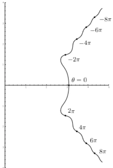
can never be a standard WKB turning point problem, like that of the Airy equation or that of the Weber equation. To visualize the situation let us show Figure A.3 which illustrates the locus of z(x) = ζ(x)⁻¹, i.e., the in- verse of a characteristic root ζ(x) of the characteristic equation of (0.11), that is, γ²expx² − U(ζ(x)⁻¹) = 0, supposing that x = x_B + rexp(iθ) (r= 0.1,−10π < θ <10π).

An important point to be observed in Figure A.3 is that, whilez(x) be- haves approximately like a constant multiple of (x−x_B)^−1/2 for|θ|small (to be more precise, for |θ| < 0.45π(< π/2), as our explicit computer-assisted computation indicates), the behavior of z(x) suddenly changes as |θ| ap- proaches the valueπ/2. In particular, the value ofz(x) for θ=±2π,±4π,· · · differs very much from z(x_B). (Cf. [AKKT3].) Thus we clearly see that the structure of the Berk-Book equation (0.11) near x_B should be completely different from that of the Airy equation, although at first sight (i.e., if we study the equation only for |θ| ¿π/2) it might appear to be approximately the same as that of the Airy equation. Furthermore a more careful and de- tailed study of the locus of z(x) with different r’s gives us Figure A.4. See [KoT] for the more detailed study of several aspects of the behavior of z(x) and some other related functions which Landau ([L]) studied in analyzing

Figure A.3: Locus ofz(x) for x=x_B+re^iθ with r= 0.1.

the penetration of an external electric field into the plasma.

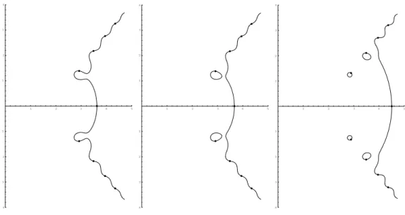
The comparison of the two figures “left” and “middle” of Figure A.4 indicates that there exist turning points of the equation (0.11) in the region {x; 0.064 < |x−x_B| < 0.066}. We note that, if x = x_∗ is a turning point of (0.11), so is its complex conjugate x=x∗ since U(z) is real-valued on the real axis. Thus it is expected that there are two turning points x₁ and x₁ in {x; 0.064 <|x−x_B| < 0.066}. In a similar manner we can find another pair of turning points x2 and x2 in {x; 0.040 <|x−xB|<0.042}, although the figure for r = 0.042 is omitted in Figure A.4 to save the space. (More careful numerical study shows thatx₁ (resp., x₂) is approximately 1.04863 + 0.0425103i (resp., 1.02429 + 0.0339953i).) This procedure of finding pairs of turning points can be continued further and such a computer-assisted study of the function z(x) strongly suggests that the point x_B is an accumulation point of turning points of the equation (0.11). This observation was the starting point of this Appendix, and we can really validate this observation by the following

Proposition A.1. Let P(X, z) denote

(A.4) U(z)−(1 + 2X),

whereU(z)is the entire function given by(A.2). Then there exists a sequence

Figure A.4: Locus of z(x) with different r’s (r = 0.066 (left), r = 0.064 (middle) and r= 0.040 (right)).

of points (X_n, z_n) (n≥1) that satisfies the following:

P(X_n, z_n) = ∂P

∂z(X_n, z_n) = 0, (A.5)

∂P

∂X(X_n, z_n)6= 0, (A.6)

∂²P

∂z²(X_n, z_n)6= 0, (A.7)

Xn→0.

(A.8)

In fact, if we set

(A.9) X=γ²(expx²−expx²_B)/2,

the pointxncorresponding toXnclearly converges toxBwith an appropriate choice of its sign. Hence Proposition A.1 entails the following

Theorem A.1. Let D(x, η(_dx^d)⁻¹) denote the Berk-Book operator, that is, (A.10) U(η( d

dx)⁻¹)−γ²expx²(=U(η( d

dx)⁻¹)−1−γ²(expx²−expx²_B)).

Then there exists a sequence {xn}n≥1 of simple turning points of the Berk- Book operator which converges to x_B.

Remark A.1. As is shown in Lemma A.3 below (cf. (A.52)), the characteristic valueζn= 1/znof the turning pointxntends to 0 asxntends toxB. This fact clearly explains why the analysis of the Berk-Book operator is so difficult at x_B. (Recall that a point (x, ζ) with ζ = 0 is outside the domain of definition of a microdifferential operator in general.)

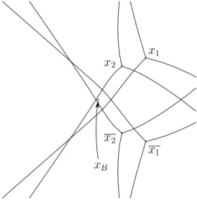
For the reference of the reader we present Figure A.5 which describes the Stokes curves for the Berk-Book operator that emanate from x₁, x₁, x₂ and x₂. (As in Figure A.2, two Stokes curves sit on the same curve in Figure A.5 also.) We refer the reader to [KoT] for a more complete study of the Stokes geometry of the Berk-Book equation nearx_B, which includes the added new Stokes curves. (See [AKKT2] for the notion of a new Stokes curve.)

Figure A.5: Stokes curves emanating from x1, x1, x2 and x2 (in the region {x; |Re(x−x_B)|<0.1,|Im(x−x_B)|<0.1}).

Let us now prove Proposition A.1. Since the argument is rather entangled, we divide it into several steps. We note that a crucially important point in our reasoning is Lemma A.2 below; there exist infinitely many pointsz_nwith

|argz_n|< π/4 such that exp(−z²_n) is fairly large, i.e., of the magnitude z_n^−k. First we note the following Lemma A.1.