Borel summability of WKB theoretic transformation to the Weber equation (Recent development of microlocal analysis and asymptotic analysis)

(1)

Abstract

We take a Schr\"odinger equation which has a pair ofsimple turning points connected by a

Stokes line, and considerWKB theoretic transformation series to the Weber equation. Under suitable conditions, the transformation series is Borelsummable, andanalysisof so-called fixed

singularities can be reduce tothe Weber equation.

\S 1.

Introduction

We consider a second order linear differential equation with

a

large parameter

(1.1) $( \frac{d^{2}}{dx^{2}}-\eta^{2}Q(x))\psi=0.$

The coefficient $Q(x)$ is

a

holomorphic function (typically rational function or

polyno-mial). $Tbe$ equation has formal solutions (WKB solutions) of the form

(1.2) $\psi(x, \eta)=\exp(\int^{x}S(x, \eta)dx)$ ,

where $S(x, \eta)=\eta S_{-1}+S_{0}+\eta^{-1}S_{1}+\cdots$ is

a

formal power seriessatisfying the Riccati

equation

(1.3) $S^{2}+ \frac{dS}{dx}=\eta^{2}Q(x)$.

The WKB solutions $\psi(x, \eta)$ $(or S(x, \eta))$ are divergent in general, and we apply Borel

resummation method. (See e.g., [12], [9].) Under generic assumptions, the WKB

solu-tions (ofsuitable normalization) is Borel summble (see [4], [8]), but in some

cases

not.

2010Mathematics Subject Classification(s): Primary $34M60$; Secondary $34M25.$

Key Words: exact WKB analysis, fixed singularity, transformationseries, Borel summability Supported by JSPS Grants-in-Aid No.22-1398

(2)

SHINJI SASAKI

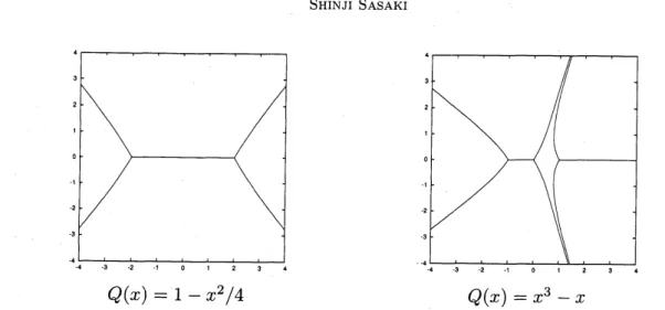
$Q(x)=1-x^{2}/4 Q(x)=x^{3}-x$

Figure _{1. two examples in which Stokes lines connect simple turning} _points

For exampleif $Q(x)=E-x^{2}/4$ _(namely _{the Weber} _{equation) with}

_a

_positive _constant

$E>0$, WKB solutions

are

not Borel summable (depending on the normalization). See

e.g., [11]. This is

a

general phenomenonif theequation hasapairof turing points (zeros

of $Q(x))$ connected by

a

_Stokes _line $\Im\int^{x}\sqrt{Q(x)}dx=0$. See e.g., [2], [3]. In Figure 1,

we

give examples of

Stokes

lines connecting turning points.

In such

cases,

_{the Borel transform of}

_a

_{WKB solution has singularities}

_on

_{the real}

axis (in the Borel plane), which we call “fixed singularites” Theyare fixed in the sence

that the location is independ of$x$

.

To analyze such singularities, in [1], WKB theoretic

transformation to the Weber equation is constructed, and Borel transformability is

given. Here transformation series is a formal power series $x(q, \eta)=x_{0}(q)+\eta^{-1}x_{1}(q)+$

$\eta^{-2}x_{2}(q)+\cdots$ which transforms the equation

(1.4) $( \frac{d^{2}}{dq^{2}}-\eta^{2}Q(q))\psi=0$

to the Weberequation (withan infinite power series $E=E(\eta)=E_{0}+\eta^{-1}E_{1}+\eta^{-2}E_{2}+$

$)$

(1.5) $( \frac{d^{2}}{dx^{2}}-\eta^{2}(E-\frac{x^{2}}{4}))\phi=0,$

with a gauge transform $\psi=x^{-1/2}\phi$. This is equivalent to _that $x(q, \eta)$ satisfies the

following:

(1.6) $Q(q)=( \frac{dx}{dq})^{2}(E-\frac{x^{2}}{4})-\frac{1}{2}\eta^{-2}\{x;q\}.$

Here $\{x;q\}$ is the Schwarzian derivative. Though this is a transformation _between

equations, this also connect WKB solutions of certain normalization. (See [1] and the

following section.)

(3)

given elsewhere.

\S 2.

Borel summability of transformation series

In this section, for simplicity

we

assume

that the

coefficient

$Q(q)$ in (1.4) is

polyno-mial. Let $q\pm$ be simple tuming points of the equation (1.4). Assume $q\pm$

are

connected

by

a

Stokes line and theother Stokes lines emanating fromthe two points tend to

infin-ity. For example, if $Q(q)=q(q^{2}-1)$ and

we

take$q+=0$ and$q_{-}=-1$, these conditions

are

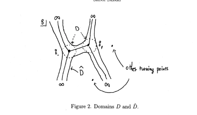
satisfied (See Figure 1). Take a neighborhood

(2.1) $D= \{|\int_{q+}^{q}\sqrt{Q}dq|<d\}\cup\{|\int_{q-}^{q}\sqrt{Q}dq|<d\}$

of $\{q_{\pm}\}$ and set

(2.2) $\hat{D}=\bigcup_{q\in D}\{\Im\int_{q}^{q}\sqrt{Q}dq=0\}.$

(cf. Figure 2.) We take $d$ small enough

so

that $\hat{D}$ does not contain any tuming points

except for $q\pm\cdot$ Then there exist formal power series $x(q, \eta)=x_{0}(q)+\eta^{-1}x_{1}(q)+$

$\eta^{-2}x_{2}(q)+\cdots$ and $E(\eta)=E_{0}+\eta^{-1}E_{1}+\eta^{-2}E_{2}+\cdots$ with $x_{j}(q)$ being holomorphic

on

$\hat{D}(j=0,1,2, \ldots)$ which satisfy the equation (1.6) and $dx_{0}/dq\neq 0.$ $x(q, \eta)$ and $E(\eta)$

are uniquely determined up to the choice of$x_{0}(q)$.

See

[1], [9].

Remark. $x_{0}(q)$ is amap which maps aturning point to a turning point, a level

curve

(Stokes line) $\Im\int^{q}\sqrt{Q}dq=0$ to a level

curve

(Stokes line)$\Im\int^{x}\sqrt{(E_{0}-x^{2}/4)}dx=0.$

There

are

two turning points $q\pm$, and

we

have two choices of$x_{0}(q)$.

The Borel summability of$E(\eta)$ is known. See [8]. In addition

we

havethe following

theorem.

Theorem 2.1. Under the assumptions above, the

_{transformation}

series $x(q, \eta)$ is

(4)

SHINJI SASAKI

Figure 2. Domains $D$ and $\hat{D}.$

Thus the equation (1.4) on $\hat{D}$

is transformed to the canonical equation (1.5) by two

Borel summable series $x(q, \eta)$ and $E(\eta)$. Then as is explained in [1] and [9] (though

mainly Airy case, not Weber case), a WKB solution of (1.4) is also transformed into

a

WKB solution of (1.5); Let $\psi(q, \eta)$ be a WKB solution of (1.4) normalized at

$q+$ $\phi(x, E, \eta)$ be

a

WKB solution

of (1.5) normalized at $2\sqrt{E}$. Here

we assume

_{$x_{0}(q_{+})=$}

$2\sqrt{E_{0}}$. (For normalization, see e.g., [9].) Then the following relation holds:

(2.3) $\psi(q, \eta)=(\frac{dx}{dq}(q, \eta))^{-1/2}\phi(x(q, \eta), E(\eta), \eta)$.

Though this is

a

formalrelation, if Borel transformed, this becomes

an

analytic relation.

Set $x(q, \eta)=x_{0}(q)+X(q, \eta)$ and $E(\eta)=E_{0}+F(\eta)$. By Taylor expansion, we have

$\psi(q, \eta)=(\frac{dx}{dq}(q, \eta))\sum_{n=0}^{-1/2\infty}X^{n}(q, \eta)\partial^{n}\phi n!$_{$\overline{\partial x^{n}}(x_{0}(q), E(\eta), \eta)$}

(2.4)

$=( \frac{dx}{dq}(q, \eta))\sum_{n=0}^{-1/2\infty}\frac{X^{n}(q,\eta)}{n!}(\sum_{m=0}^{\infty}\frac{F^{m}(\eta)}{m!}\partial E^{m}\partial x^{n}\partial^{n+m}\phi(x_{0}(q), E_{0}, \eta))$ .

Then by Borel transform,

we

have

(2.5)

$\psi_{B}(q, y)=((\frac{dx}{dq})^{-1/2})_{B}(q, y)*\sum_{n=0}^{\infty}\frac{X_{B}^{*n}(q,y)}{n!}*(\sum_{m=0}^{\infty}\frac{F_{B}^{*m}(y)}{m!}*\frac{\partial^{n+m}\phi_{B}}{\partial E^{m}\partial x^{n}}(x_{0}(q), E_{0}, y))$,

where the subscript $B$

means

Boreltransform _$and*$ is convolution. Now let us takeone

term

$(( \frac{dx}{dq})^{-1/2})_{B}(q, y)*\frac{X_{B}^{*n}(q,y)}{n!}*\frac{F_{B}^{*m}(y)}{m!}*\frac{\partial^{n+m}\phi_{B}}{\partial E^{m}\partial x^{n}}(x_{0}(q), E_{0}, y)$ .

(5)

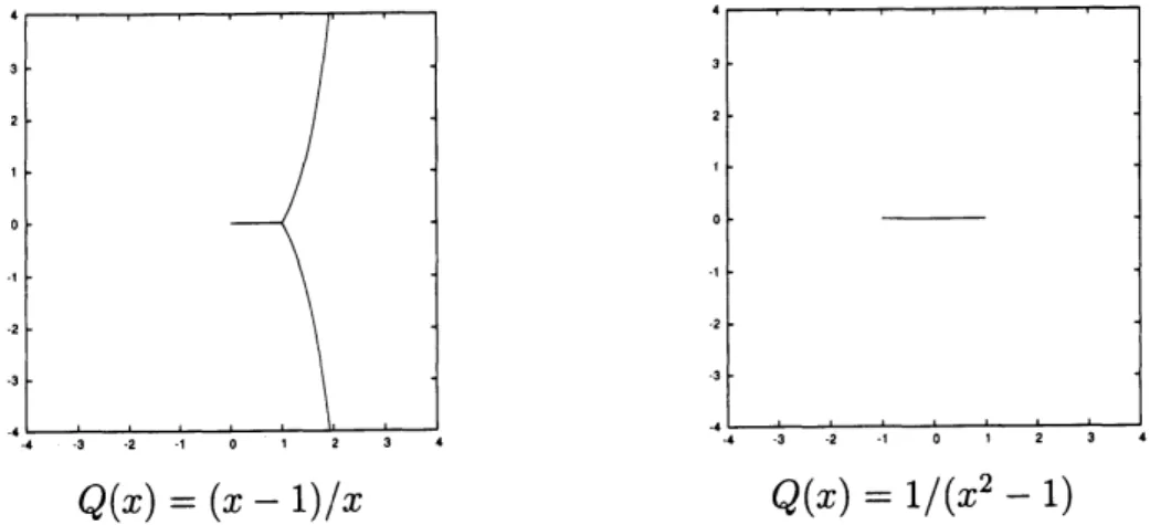
$Q(x)=(x-1)/x Q(x)=1/(x^{2}-1)$

Figure

3.

Stokeslines connecting

a

pairof

a

simple turning pointand

a

simplepole(left),

a

pair ofsimple poles (right).

Since $X$ and $F$

are

Borel summable, the front part

$(( \frac{dx}{dq})^{-1/2})_{B}(q, y)*\frac{X_{B}^{*n}(q,y)}{n!}*\frac{F_{B}^{*m}(y)}{m!}$

is holomorphic in

a

strip region containing the positive real axis. Since

we

know well

about $\phi_{B}$ (see e.g., [11], [10]), for this single term,

we

can see

continuability avoiding

singularities, disconitinuity at

a

singularity, etc. Then by summing up with respect to

$m$ and $n$ (with

care

on convergence), we see continuablity etc. also for $\psi_{B}(q, y)$.

Remark. $\phi_{B}(x_{0}(q), E_{0}, y)$ has infinitely many singularites in the $y$-plane with real

period$2\pi E_{0}$, and with Borel summability

we can

analyze all singularitiesthrough

trans-formation. Thus Borel summability of transformation is important in the analysis of

fixed singularities.

Remark. In this paper, we considered only two simple turning points problem. On

the other hand, simple poles (of $Q$) are known to play

a

role similar to simple turning

points ([6], [7]), and

a

pair of

a

simple turning point and

a

simple pole,

or a

pair

of

simple poles

causes

fixed singularities

as

well (cf. Figure 3). The former one can be

treated in the

same manner as

a pair of simple turning points. However the latter

one

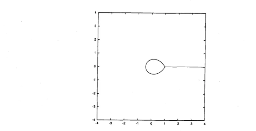
is difficult to treat with. Also, a sole simple turning point makes a pair in

some

sense,

(6)

SHINJI SASAKI

Figure 4. $A$ loop of

Stokes

line ending

a

sole simple tuming point.

References

[1] Aoki, T., Kawai, T. and Takei, Y., TheBender-Wu analysis and the Voros theory, Special

Functions: ICM-90 Satellite

_Conference

Proceedings (M. Kashiwara and T. Miwa, eds),

Springer-Verlag, 1991, pp. 1-29.

[2] Delabaere, E., Dillinger, H. and Pham, F., R\’esurgence de Voros et p\’eriodes des courbes

hyperelliptiques, Ann. Inst. Fourier (Grenoble) 43 (1993), 163-199.

[3] Delabaere, E. and Pham, F., Resurgent methods insemi-classical asymptotics, Ann. Inst.

Henri _Pincare 71 (1999), 1-94.

[4] Dunster, T. M, Lutz, D. A. and Sch\"afke, R., Convergent Liouville-Green expansions for

second-order linear differential equations, with an applition _{to Bessel functions, Proc. R.}

Soc. Lond. Ser. A Math. Phys. Eng. Sci. 440 (1993), 37-54.

[5] Kamimoto, S. and Koike, T., Onthe Borel summability_{of WKB-theoretic transformation}

series, RIMSpreprint 1726 (2011).

[6] Koike, T., Onaregular singular point in the exactWKB analysis, Toward the Exact WKB Analysis

_{of Differential}

Equations, Linear

_of

Non-Linear (C. J. Howls, T. Kawai and Y. Takeieds.), Kyoto Univ. Press, 2000, pp. 39-54.

[7] Koike, T., On_{the exact WKB analysis of second order linear ordinary}_differential_equations

with simple poles, Publ. Res. Inst. Math. Sci. 36 (2000), 297-319.

[8] Koike, T. and Sch\"afke, R., in preparation.

[9] Kawai, T. and Takei, Y., Algebraic Analysis

_of

Singular Perturbation Theory, Transl.

Math. Monogr. 227, Amer. Math. Soc., 2005.

[10] _{Sasaki, S., Resurgence of WKB solutions of the Weber} _equation _{through integral}

repre-sentation, in preparation.

[11] Takei, Y., Sato’s conjecture for the Weber equation and transformation theory for Schr\"odinger equations with a merging pair of turning points,

_Differential

Equations and Exact WKB Analysis (Y. Takei, ed), RIMS K\^oky\^uroku Bessatsu B10, 2008, pp. 205-224.

[12] _{Voros, A., The return of the}_quartic _oscillator–The complex WKB method, Ann. Inst.

Henri Pincare 39 (1983), 211-338.