Japan Advanced Institute of Science and Technology, in partial fulfillment of the requirements

Japan Advanced Institute of Science and Technology

JAIST Repository

https://dspace.jaist.ac.jp/

Title Collision Avoiding Motion Planning of Autonomous Robots with MANETs

Author(s) 岡田, 崇

Citation

Issue Date 2007‑03

Type Thesis or Dissertation Text version author

URL http://hdl.handle.net/10119/3616 Rights

Description Supervisor:丹 康雄, 情報科学研究科, 修士

Collision Avoiding Motion Planning of Autonomous Robots with MANETs

By Takashi Okada

A thesis submitted to School of Information Science,

Japan Advanced Institute of Science and Technology, in partial fulfillment of the requirements

for the degree of

Master of Information Science

Graduate Program in Information Science

Written under the direction of Associate Professor Yasuo Tan

March, 2007

Collision Avoiding Motion Planning of Autonomous Robots with MANETs

By Takashi Okada (510021)

A thesis submitted to School of Information Science,

Japan Advanced Institute of Science and Technology, in partial fulfillment of the requirements

for the degree of

Master of Information Science

Graduate Program in Information Science

Written under the direction of Associate Professor Yasuo Tan

and approved by

Associate Professor Yasuo Tan Professor Yoichi Shinoda

Associate Professor Mikifumi Shikida

February, 2007 (Submitted)

Copyright c2007 by Takashi Okada

Abstract

In the research topic of large scale autonomous networked mobile robots, the experiment is difficult in various aspects. On the purpose of constructing above system, at first this research mentions the experiment platform which supports above condistions. Next it mentions the mothion planning algorithm which suits these case.

Contents

1 Introduction 6

2 Related Works 7

2.1 Motion Planning . . . 7

2.2 Robot Implementation . . . 10

3 Motion Planning 11 3.1 Path Planning in Expansive Configuration Spaces . . . 11

3.1.1 Expansion . . . 11

3.1.2 Connection . . . 12

3.2 Proposed approach . . . 13

3.2.1 Definitions . . . 13

3.2.2 New Expansion . . . 13

3.2.3 New Connection . . . 15

3.2.4 Prioritized Planning . . . 16

3.2.5 Algorithm . . . 17

4 Experiment Platform 18 4.1 Overall Architecture . . . 18

4.2 Hardware Emulation . . . 20

4.3 Network Emulation . . . 20

4.4 WLAN Emulation : QOMET . . . 22

4.5 Experiment Integration : RUNE . . . 23

5 Robot Applications 25 5.1 Application Messages . . . 25

5.2 Application Flows . . . 25

6 Experiment 32 6.1 Experiment Definitions . . . 32

6.1.1 Emulated Environment Definition . . . 32

6.1.2 Emulated Robot Definition . . . 33

6.1.3 Scenario Definitions . . . 34

6.2 Experiment Results . . . 36

1

6.2.1 Simple Scenarios . . . 36 6.2.2 Scenario 3 : 10 Robots Scenario . . . 37 6.2.3 Large Scale Scenario . . . 38

7 Discussions 41

7.1 Motion Planning . . . 41 7.2 Experiment Platform . . . 44 7.2.1 Evaluation of the Experiment Platform . . . 44

8 Future Works 46

8.1 Implementation of MANET protocols . . . 46 8.2 Experiment Framework . . . 48 8.2.1 StarBED2 . . . 48

9 Conclusions 52

A Communication between Map Manager and Robots 54 A.1 Initialization of Map Manager . . . 54 A.2 Initialization of Robots . . . 55

B Configure dummynet 56

B.1 Making a new pipe . . . 56 B.2 Configure a pipe . . . 57 B.3 Remove a pipe . . . 57

C Integration with RUNE 58

2

List of Tables

5.1 Map Manager Message . . . 26

5.2 Robot Management Message . . . 26

5.3 Robot Application Message . . . 27

5.4 the parameters of setting of robot . . . 27

6.1 the parameters of QOMET . . . 33

6.2 the connection ranges from QOMET . . . 33

6.3 the parameters definition of the robot . . . 34

6.4 Scenario 1 : One robot and one obstacle . . . 35

6.5 Scenario 2 : Two robots . . . 35

6.6 Scenario 3 : Ten robots and six obstacles . . . 36

6.7 Scenario 4 and 5 : Fifty and a hundred robots . . . 36

7.1 Comparison Experiment platform . . . 45

3

List of Figures

2.1 Find a path from Roadmap . . . 8

3.1 Expansion . . . 12

3.2 Connection . . . 13

3.3 New Expansion . . . 14

3.4 New Connection . . . 16

4.1 Emulation on StarBED . . . 19

4.2 Hardware Emulation Architecture . . . 20

4.3 Map Manager Architecture . . . 21

4.4 General System Overview . . . 22

4.5 Two-state WLAN emulation . . . 22

4.6 Structure of experiments using RUNE. . . 24

5.1 Flowchart of General Applications . . . 28

5.2 Flowchart of Map Manager. . . 29

5.3 Flowchart of Robot . . . 30

5.4 Flowchart of Planning . . . 31

6.1 Scenario 3 : Ten robots and six obstacles . . . 35

6.2 Robot trajectory of Scenario 1 : One robot and one obstacle . . . 37

6.3 Robot trajectories of Scenario 2 : Two robots . . . 38

6.4 Robot trajectories of Scenario 3 : Ten robots and six obstacles with Algo- rithm 1 . . . 39

6.5 Robot trajectories of Scenario 3 : Ten robots and six obstacles with Algo- rithm 2 . . . 39

6.6 Robot trajectories of Scenario 4 : Fifty robots and twenty obstacles . . . . 40

6.7 Robot trajectories of Scenario 5 : A hundred robots and forty obstacles . . 40

7.1 Total time from src to dst each Algorithm . . . 42

7.2 Waiting time and turning number of Algorithm 1 . . . 43

7.3 Waiting time and turning number of Algorithm 2 . . . 44

8.1 The problem of MANET emulation . . . 47

8.2 The problem of MANET emulation . . . 48

8.3 Application forwards messages . . . 49 4

8.4 Apply configurations at once . . . 50

8.5 Town emulation by StarBED2 . . . 51

C.1 Logical structure of RUNE . . . 60

C.2 Logical structure of RUNE . . . 61

5

Chapter 1 Introduction

In disaster area or office building, autonomous robots act instead of human beings. Rescue robots are able to accomplish many tasks in dangerous places where humans cannot enter, such as sites where harmful gases or high temperature are present, the hard environment for human. Cleaning robots can also work automatically and save costs by performing various routine tasks. In all these examples robots have to move to their destination in order to perform their function. For this purpose they need to be able to recognize the changes of environment around them and equip a motion planning method in order to avoid obstacles which have probability making collision with them.

In this research topic, the experiments for evaluating such researches are difficult, since the cost of these real autonomous robots is high. This is particularly true if researchers want to experiment more than a few robots, and need to test systems with tens or even hundreds of robots. Then many researchers try to make experiments or evaluate their algorithms or methods on software simulators. But the results from these simulators are not really precise. The difference between real system and simulators is much big. In real environment, many kinds of noise affect conditions. For example, the connection on real environment is affected by electric waves and magnetic field and so on. Researchers can not always obtain good results on real system, even if they have once obtained good results from experiments on simulators. Then the system needs some solutions on purpose of covering this difference.

In this paper, I propose an experiment platform which large number of autonomous mobile networked robots are executed. And to fulfill it, I propose an new algorithm of motion-planning as an application.

6

Chapter 2

Related Works

In this chapter, at first one of popular motion-planning method is introduced. Next is the experiment platform which enables researchers to perform and evaluate their researches.

2.1 Motion Planning

In the situation that multiple robots act in same environment, they need navigation in order to move to their destination on purpose of accomplishing their tasks and avoid possible collisions with other robots or obstacles. Multiple robot motion planning are usually classified as centralized or decentralized method. Centralized planners construct plans by one robot and this robot distributes the plan. In Decentralized method, each robot plans independently.

One of traditional way is sampling based motion-planning [2]. In this approach, sam- ples are organized into regular grids or hierarchical ones. These grids express the location of the free space. And the planner remember these locations where robots already vis- ited. But the size of these grids increases exponentially according to the dimension of the configuration space, for example the number of degrees of freedom of the robot. Then the calculating the free configuration space takes high cost, if the dimension of the configu- ration space is more than four or five.

A probabilistic roadmap (PRM) planner has become popular method in these planning case because of the speed of calculation. Many of PRM planner of multiple robot are decentralized. Basic PRM executes the following steps :

PRM planner method

Roadmap Generation

At first the planner selects some milestones from configuration space at random.

And next the planner tries to joint each neighborhood if the path between each neighborhood is collision-free.

Roadmap Extension

7

The planner tries to joint each roadmap created. If the roadmaps could not joint with them, it tries random-walk between each roadmaps which could not joint.

Route Search

If the planner can joint the constructed roadmap with the source and the destination, then searches a shortest path using Dijkstra’s algorithm.

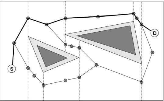
Figure 2.1 describes one simple example of constructing a roadmap. As described in the figure, S is a source of a robot and D is a destination, triangles of dark grey color are shape of obstacles and light colors means the space where a robot makes collision if it enters the range. Then at first of path-planning the entire map is divided into trapeziums. This rule of divisions draws perpendicular lines from vertices of all obstacles.

Next it puts milestones on the center of these perpendicular lines and on the center of the trapeziums, and connects these milestones. Finally Sand D connects the milestones in same trapeziums and a path is found.

S

D

Figure 2.1: Find a path from Roadmap

A PRM planner randomly samples the configuration space of robots and register the collision free samples as milestones. And the planner tries to connect pairs of these mile- stones and saves this collision free connections as the trajectories of robots. Probabilistic

8

roadmap means this graph, the edges are the trajectories of robots, the nodes are the mile- stones, and the undirected graph jointing the trajectories is the probabilistic roadmap.

And the planner finds the optimal path from the graph, for example it may set some weights on these edge and use Dijkstra’s algorithm.

PRM planners are not complete in the traditional sense. But they are probabilistically complete under certain assumptions. It means that the probability of failure decreases exponentially to zero with iterations [3].

Now I mention two types of PRM, one is single-query planners. It computes a new roadmap from scratch for each new query [3]. Second one is multi-query. It precomputes the roadmap and re-use the roadmap for answering queries [9]. It has been proven that, under reasonable assumptions about the geometry of the robot’s configuration space, a relatively small number of milestones picked uniformly at random are sufficient to capture the connectivity of the configuration space with high probability.

In addition to PRM method, robots need technique which avoid collisions of each robot.

Simply if robots exchange their trajectories and start to plan, this method does not care about the trajectories of each other. ”Velocity turning” [13] method computes the relative velocities of the robots to avoid inter-robot collision. Another way to solve this problem is ”Prioritized Planning” [14]. The robots avoid possible collisions depending on their priority.

9

2.2 Robot Implementation

When researchers are implementing or evaluating something related to autonomous robots, for example path planning algorithm or dynamic network construction and so on, one of the choices is simulation, by using a product such as Webots [10], co-developed by the Swiss Federal Institute of Technology in Lausanne, Switzerland. Software simulator mod- els robot components, networks and motions and time scheduling and surrounding envi- ronment. If researchers select to use such simulators, they have to implement simulator- specific modules by themselves. Surely these software simulators can test various kinds of environment that it is hard to implement in a real system. But the results from these software simulators may differ with respect to those that would be observed in a real system. It means that the difference between the results from software simulator and results of a real system is maybe much larger.

The second one is to implement on real environment. RoboCup [5] involves teams of five small robots, each up to 18cm in diameter and 15cm in height. The robot teams are entered into a competition to play soccer against opponent teams fielded by other research groups. Hsu [7] made experiments on his research team testbed. This robots move frictionlessly on an air bearing on a 3 m x 4 m table. ARL (Stanford Aerospace Robotics Laboratory) citeStanford makes various experiments of real robots. These real environment systems take much cost for real robots and sensing. If researchers want to test large number of robots, it is hard to make the ready all robot hardware equipping an ability to compute and connect wireless network.

Third one is emulation. The difference between simulation and emulation is like the difference between modeling and emulation. A simulation is a modeling system out of approximations or inferences. An emulation is emulating or imitating a different environ- ment of hardware or software. This method can not only get reliable experiment results but also not take much cost. If researchers can emulate robots and other environment on computers, the const is only computers. And this approach covers the gap between real implementation and software simulation. StarBED [8] is a large scale, realistic and real time network testbed, using hundreds of PCs, and switched networks. StarBED2 [18]

expands StarBED so as to be suitable for emulating ubiquitous networks.

10

Chapter 3

Motion Planning

As mentioned already, one of the essential feature of autonomous mobile robots is a motion-planning algorithm. Autonomous robots need some path-finding algorithm to avoid probability which cause collisions with robots or obstacles.

Many path-planning algorithms have been proposed to date. The performance of motion-planning algorithm can be characterized by the following properties: speed, com- pleteness, and optimality. In dynamic and unknown environment, robots must plan and re-plan their motion many times, because the environment dynamically changes in time.

Therefore in the case when robots need to continuously plan on-the-fly their trajectory, the algorithm speed is one of the most important properties.

3.1 Path Planning in Expansive Configuration Spaces

In proposed system, robots equip a kind of PRM method that base on ”Path Planning in Expansive Configuration Spaces” [3]. The definitions of this algorithm are the following.

For example, a configuration can be specified bydparametersq = (q0, q1,· · ·, qd−1), where d is the number of defined degrees of freedom of a robot. The set of all configurations forms the robot’s configuration space C. A configuration q is free if the robot placed at q does not collide with obstacles. The basic idea of this paper is using single-query path planning methods, there are given two configurationsqsource and qdestination. They sample at random from configuration space C and register only q that have collision-free path

fromqsource orqdestination. Then they grow two trees from qsource or qdestination. These two

trees keep on building till accomplishing the connection both q of these two trees with collision-free.

This algorithm iteratively executes two basic steps, expansion and connection until either a path is found or the maximum number of iterations is counted.

3.1.1 Expansion

Expansion is the first step of this planner, by which the planning method build two trees Tsource = (Vsource, Esource) andTdestination = (Vdestination, Edestination).

11

Src Dst Candidates ExpansionRange

Figure3.1:Expansion

Figure3.1describesthisappearance.Thesetwooperationsoftreesareidentical,andextendtreeT=(V,E)startingfromtherobotinitialposition(source)andtherobotdestination,respectively.Whenbuildingeachofthesetrees,theplannerpicksupanodexfromexistingmilestones,whichischosenwithaprobabilityproportionalto1/w(x).Thevalue1/w(x)representstheweightofnodex,anditisequaltothenumberofneighborsofxplus1(thenodexitself).Thelargerthenumberofneighborhoodofthenodexis,themorethenodexisselected.Aftertheplannerselectedanodex,ittriestopicksomecandidatesofmilestonestoexpandthetree.Andtheplanneraddsthemtothetree,ifthosecandidatesareeffectivelyreachablefromx.

3.1.2 C onnection

Connectionisthesecondstepofthealgorithm,inwhichthisplannertriestoconnectthetwopreviouslybuilttrees,TsourceandTdst.

Figure3.2describesthesituationwhichtwotreesconnecttoeachother.Thiscon-nectionmethodissimple.Foreverynodesinthesetofverticesofthecorrespondingtrees,VsourceandVdestination,forexamplexispickedfromVsourceandyispickedfromVdestination,theplannercheckswhethertheseverticescanseeeachotherornotandcheckwhetherthedistancethatitissmallerthandistance(x,y)ornot,andiftheplannerfindtwomilestoneswhichsatisfytheaboveconditionsfromeverytreeandtheedgeiscollisionfree,theplannerterminatessuccessfully.

12

Source Destination

CONNECT Connect Expand

Figure3.2:Connection

3.2 P rop o sed a pproa c h

Inthecasestudyofthispaper,robotsareconsideredtobeplacedinenvironmentthatareunknownorchangeinadynamicmanner.Themotion-planningmethoddescribedabovedoesnotsuitesuchacase.Forexample,thepreviousplannercannotpredictwhetherthereareanycollisionsornotinthetreebuiltfromdestination,Tdestination.Itmeansthattheplannerhasnowaytoknowthetimewhentherobotwillreachthemilestonesinthetree,Tdestination.Hencetheplannercannotexpandthetree,Tdestination,inthesecases.Inordertoadapttheplannertotheseconditionsofunknownanddynamicenvironment,thenotionofthetimeisimportantinthesecases.Becauseeveniftheplannerfoundsomepathtodestination,thepathmightbeinefficientwithmuchcalculatingtime.Indynamicenvironment,robotshavetoplantheirpathinrealtime,itisimportantthatthetimekeepsonrunningduringplanningnewpath.AndIadaptedthemotion-planningmethoddiscussedinthefollowingsections.

3.2.1 D efinitions

Atfirsttheparametersofthismotion-planningmethodshouldbedefined.ThedefinitionsofqandCaresimilartoSection3.1.Theparameterqistheelementofdegreeswhichrobotscanmovefree.Cistheconfigurationspace,meansallthesetofthisq.Aconfigurationsqisfreeiftherobotplacedatqdoesnotcollidewithobstacles.ThesetofallfreeconfigurationsaredefinedthefreespaceF.

3.2.2 N ew Expansion

Asmentionedabove,inunknownanddynamicenvironment,introducedpath-planning[3]doesnotworkwell.Thenmyalgorithmusesfollowingmethod:

13

Src

Obstacle Candidates

Configurationtime space ExpansionRange

Another Robot

Figure3.3:NewExpansion

Growsonlysourcetree

Thismeansthattheplannergrowsonlyonetree(Tsource),thisiswhytheplannercannotcheckthecollisionsofTdestination.Thismethodisdiscussedin[3],buttheyrecommendthiswayonlywhentherobotishighlyconstrainedaroundqsourceorqdestination,thenavoidtogrowthetreefromthisconstrainedq.

Adapttimeparameter

Themilestoneshavethetimeparameterwhentherobotsreachtothemilestone.Ifmilestonesdonotincludethisvalue,theplannercannotpredictthecollisionwithotherautonomousmobilenetworkedrobotsorobstacles.ThisisfulfilledbyConfigurationtimespace.Itisakindofconfigurationspacebutincludingthetimeparameter.Figure3.3describesthis.Thisconfigurationspacecoverstheothermovingrobotsasmovingobstacles,andtherobotsavoidtopickthisconfiguration.

ThenIadaptaboveconditionsto”Expansion”method.

A lgorithm Exp a nsion

1.PickanodexfromVwithprobability1/w(x).

2.SampleKpointsfromNDd(x,time)={q∈C(time)|dminimum<distc(q,x)<Dmaximum},wheredistcissomedistancemetricofC(time).(KanddminimumDmaximumarepa-rameters.

14

3. for each configuration y that has been picked do

4. calculate w(y) and register y with probability 1/w(y)

5. ify is registered,clearance(y)>0 and link(x, y) return YES 6. then put y inV and place an edge between x and y. In step 1, the meaning of probability 1/w(x) is same as based method.

In step 2, K is the number which the planner tries to pick the milestones from above conditions. dminimum and Dmaximum are the minimum and maximum distance which the planner can set the candidates of milestones. Then by NN d(x), the planner picks the milestones which are plotted in the above range and are collision-free in predicted current time. C(time) is ”Configuration time space”, it is the configuration space in time.

In step 5,clearance(y) is the minimum distance, which is defined as its minimal distance to the boundary ofF. And link(x, y) is the checking whether x can ”see” y without any obstacles on its sight.

In thisExpansionphase, the constant numbers,K, dminimum, Dmaximum affect the ability of this planner. If the planner increases K, the optimality also increases but the calcu- lation costs increase too. No less than the number K, if it increase the range between

dminimum and Dmaximum, same situation causes. Then the definition of K and dminimum

and Dmaximum is much important for this motion-planning.

3.2.3 New Connection

As expressed in Expansion method, the planner tries to connect only newly added mile- stones last step.

Algorithm Connection1

1. for every newly added x∈Vsource do

2. ifdstw(x, qdestination)< l (l is a parameter.)

3. then link(x, qdestination).

In step 1, the newly addedxare the milestones which the planner added lastExpansion step. In step 2, l is some constant distance. This l also influence the planning time and the ability of this planner. If link(x, qdestination returns YES for some x, then a path is found between qsource and qdestination through x.

But there is a possibility which the algorithm run faster. Basically the robots can not know the entire map at once, but the robot use PRM planning for avoiding collisions in some complicated area. Then the idea is going straight trajectory after passing through this complicated area. This is simply realized by taking away the step2 above algorithm

15

Source Destination Obstacle Connect Expand

CONNECT

Figure3.4:NewConnection

asfollows:

A lgorithm Conne ction2

1.foreverynewlyaddedx∈Vsourcedo 2.link(x,qdestination).

3.2.4 P rioritized Planning

Inadditiontothesetwomethods,thesystemneedstocorrespondtolarge-scalemultiplerobots.Everyrobothastocommunicateandavoidpossiblecollisionswitheachotherifrobotsdetectthecollisionintheircurrenttrajectory.Thentheserobotsavoidthecollisionaccordingtothepriority,forexampletherearetworobotsAandB,andassumethepriorityofAishigherthanthepriorityofB.Nowtheirtrajectoriesmakecollisioniftheykeeponmovingtheirtrajectories.ThenrobotAkeeponitstrajectoryandrobotBneedstofindatrajectorywhichavoidpossiblecollision.Thisprioritizedplanningmeansthatthelowerpriorityrobotregardsthehigherpriorityrobotasamovingobstacle.Thentheconfigurationspaceofthislowerpriorityrobotislimited.Thislimitedconfigurationspaceis”Configurationtimespace”,andallofrobotshavetoconsidertheirtrajectoryonattentionofthislimitation.Thismeansthatthelowerthepriorityofrobotis,themoretheconfigurationspaceoftherobotdecreases.

16

3.2.5 Algorithm

By using above Expansion and Connection algorithm and Prioritized Planning, I adapt PRM planner to multiple robot in real time on unknown and dynamic environment as follows :

Algorithm1

1. Iftime < t (t is a parameter.) 2. then Expansion

3. IfConnection1 returns YES

4. then register new found path

5. Compare all found paths and return fastest path

Algorithm2

1. Iftime < t (t is a parameter.) 2. then Expansion

3. IfConnection2 returns YES

4. then register new found path

5. Compare all found paths and return fastest path

In step 1, time is current time, and t is a parameter when limit the steps which the planner executes.

In step 4, if the planner found a path between qsource and qdestination.

In step 5, the planner returns the path which the time when a robot reaches toqdestination

is earliest from all found paths.

The difference between Algorithm 1 and Algorithm 2 is only selecting which Connection method.

In this chapter, at first I introduce the based motion-planning algorithm and next, represent the problems of this algorithm in unknown and dynamic environment. After that, I propose a new algorithm which suite in these cases.

17

Chapter 4

Experiment Platform

Researchers need to confirm and evaluate the effects of their proposed research. When they implement large-scale autonomous mobile networked robots, this is very difficult phase by many reasons as follows.

If they try to evaluate their contents of researches on software simulator, there may appear big gaps when they implement on real system in next step. If they try to create real mobile multiple robots system, the costs of the various hardware are much expensive and they may encounter unexpected problems to control them.

Then emulation is one of the effective and appropriate method to implement these system. In this chapter, I propose a new experiment platform to emulate large-scale autonomous mobile networked robots.

4.1 Overall Architecture

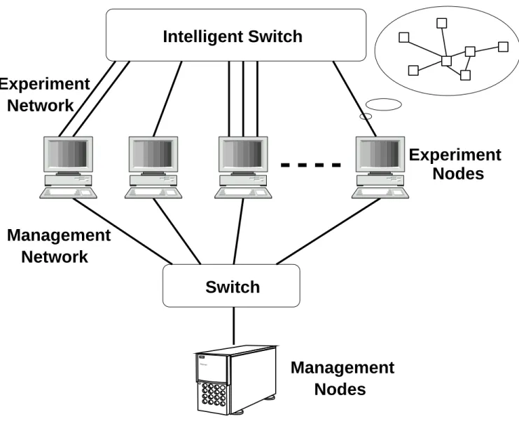
The robots in the proposed system cooperate in order to reach a destination while avoiding collisions and accomplish some given tasks. To express these large-scale robots, a suitable network testbed is needed. For this purpose I use StarBED [8]. StarBED is large- scale network testbed which has a large number of PCs (more than 700) and network interfaces. These all experiment PCs are equipped with at least two network cards (100 Mbps or 1Gbps type). These PC can easily construct large-scale networks by changing switches. All of robots are emulated on StarBED PCs and communicate through Ethernet configurations. Figure 4.1 describes the entire architecture of the system.

To fulfill executing emulated robots on StarBED, following contraptions are needed : Hardware emulation

For the system assumes real PCs to be autonomous mobile networked robots, the modeling and emulations are needed. This is given in Section 4.2

Network emulation

18

Primergy

Intelligent Switch

Switch

Nodes Management

Nodes Experiment Network

Experiment

Network Management

Figure 4.1: Emulation on StarBED

The networks of StarBED are Ethernet or 802.3 networks, these this networks also need some method to emulate WLAN communication. This is given in Section 4.3 and 4.4.

Expand into large-scale

This system executes large-scale networked robots, and to fulfill this, it needs some experiment integration method. This is given Section 4.5.

Robot application

Finally of course these robots execute applications to communicate to each other.

In this system, robots equip motion-planning (proposed in Section 3.2) application.

19

4.2 Hardware Emulation

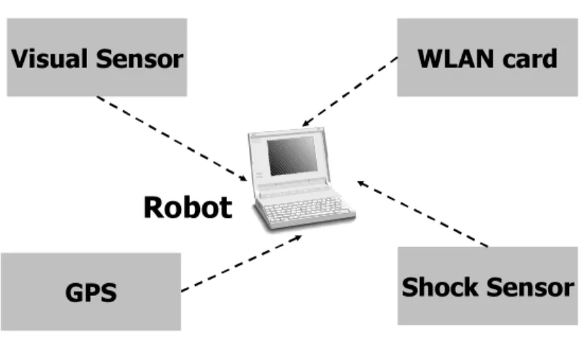
For emulating robots on StarBED PCs, the system needs some modeling to represent the hardware of robots, for example motors or some sensors and so on. In unknown and dynamic environment the system needs to know dynamic changes of environment and some structure which synchronize the events which happens on every robots in same time. In this system,Map Manageradministrates all these hardware information. Figure 4.2 describes the general overview of controlling hardware messages in this system.

Robot

GPS

WLAN card

Shock Sensor

Figure 4.2: Hardware Emulation Architecture

Each robots is able to know what happens on their hardware from the emulated hard- ware information, for example images from ”Visual sensor” or detection of WLAN radio signal or some alarm messages from ”Shock sensor” and so on. These hardware infor- mation is treated by the application of robots from the messages of ”Map Manager”, it means that this system consider these emulated hardware information to be the messages from device driver. Figure 4.3 describes the architecture of ”Map Manager”.

4.3 Network Emulation

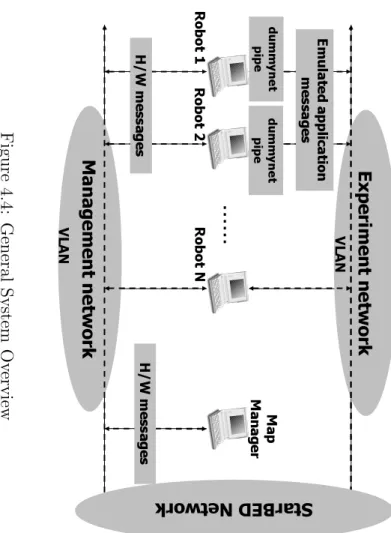
The mobile networked robots communicate on wireless network, then the system has to emulate this network system. Figure 4.4 shows the overall network architecture of this system. These two networks are separated by switching and creating VLAN, and there are two types of streams on each different networks. On ”Management Network”,

20

Robot 1Robot 2Robot N Map Manager

・・・・・・ WLAN radio

GPS InfoVisual Image : H/W information

Shock Alarm

Figure4.3:MapManagerArchitecture

themessagesofemulatedhardwareinformationwhichareshownintheprevioussectionaresent.ThisnetworkisEthernetnetworkwithoutanylimitations,andtheseemulatedhardwaremessagesareimmediatelyreceivedbyemulatedrobotPCsand”MapManager”.”ExperimentNetwork”isthenetworkwhichisassumedasrealWLANnetworkatdisasterareaorofficebuildingorhome.Therobotscommunicateandcooperatebysendingthemotion-planningmessagesthroughExperimentNetwork.

TofulfilltheWLANcommunication,thesystemapplysomeemulatedWLANcon-figurationvalues(forexample,thebandwidthorthedelayorthejitterandsoon)toEthernetcablenetwork.ThisemulationcanberealizedbyWLANemulator:QOMET[15](seeSection4.4moredetails).TheWLANcommunicationemulationengineQOMETisdeployedintheemulatedrobotstoallowrecreatingnetworkconditionssimilartothoseoccurringinarealWLANenvironment.InordertoadapttheseWLANconfigurationvaluetoEthernetcablenetwork,dummynet[16]iseffectiveineveryconstantsteps.DummynetsuppliesvariousconditionsofnetworkthroughIPqueues.Emulatedrobotsmanagesthesequeuesforeveryrobotsotherthanitself.AndthesequeueslimitthecommunicationaccordingtoWLANconfigurationvalues,asitwillbedetailedinnextsection.Inordertoimplementsuchcomplexexperimentsystem,thesystemincludesanexperiment-supportsoftware,calledRUNE(Real-timeUbiquitousNetworkEmulationenvironment)[?].Itprovidesadditionalfunctionalitywhichsupportslarge-scaleemulationsystem.Fig-ure4.6showstheintegrationwithRUNEofthissystem.TheRuneMastermanagestheentiresystem(seeSection4.5formoredetails).

21

Robot 1Robot 2Robot N Map Manager Experiment network

Management network H/W messagesH/W messages Emulated application messages

StarBEDN etwork

・・・・・・ VLAN

VLAN dummynetpipe dummynetpipe

Figure4.4:GeneralSystemOverview

4.4 W LAN E m u la tion : QOMET

Thescenario-drivenarchitectureforWLANemulationhastwostages.Inthefirststage,fromareal-worldscenariorepresentationQOMETcreateanetworkqualitydegradation(ΔQ)descriptionwhichcorrespondstothereal-worldevents(seeFigure4.5).

Figure4.5:Two-stateWLANemulation

ByqualitydegradationQOMETmeanthechangeinnetworkservicequalitybetweentwomeasuringpoints;QOMETdenotethisdegradationbytheshorthandΔQ.SincetheΔQdescriptionrepresentsthevaryingeffectsofthenetworkonapplicationtraffic,theWLANemulator’sfunctionistoreproduceit.TheΔQdescriptioncalculatedinthefirststageisthereforeconvertedintoanemulatorconfigurationthatisusedduringtheeffectiveemulationprocesstoreplicatetheuser-definedscenarioinawirednetwork.Thismakesitpossibletostudytheeffectsofthescenarioontherealapplicationundertest.This

22

WLAN emulation model is an aggregation of several models used at the various steps of the conversion of the scenario representation to the network Δ Q description which is needed to recreate those scenario conditions. The following steps describe the these models at each level of the conversion: real world scenario to physical layer, physical layer to data link layer, and, finally, data link layer to network layer. Modeling stops at network layer because it is at this level that QOMET introduce the quality degradation using a wired network emulator.

4.5 Experiment Integration : RUNE

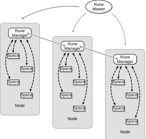
Rune(Real-time Ubiquitous Network Emulation environment) provides an API set which controls experiment environments. The fundamental function of Rune is to implement a test environment in which a number of ”spaces” that emulate each experiment target can work on either single or multiple nodes. Rune provides a reasonably abstracted interface for easily implementing emulation targets as spaces without much concern about the interaction between emulation nodes. Runehas the following roles:

• experiment environment setup/cleanup and progress management;

• procedure invocation;

• interaction between spaces;

• time synchronization;

• mutual exclusion.

Figure 4.6 shows the structure of an experiment implemented usingRune. The ”Rune Master” module manages the configuration of each experiment, and controls the progress of the experiment. The execution of all spaces deployed on multiple nodes is initiated by Rune master via modules called Rune Manager. The Rune manager is deployed on every emulation node and mediates communication between them through objects called

”conduits”. Spaces implementing emulation targets exist on emulation nodes in the form of shared objects, loaded dynamically by theRune manager.

23

Rune Manager

Space

Space

Space

Space Node

Rune Manager

Space

Space

Space

Space Node

Rune Manager

Space

Space

Space

Space Node Rune

Master

Figure 4.6: Structure of experiments usingRUNE

24

Chapter 5

Robot Applications

When researchers implement a system of autonomous mobile networked robots on their own environment, they also have to describe behaviors of robots. The robots in the system equip proposed motion-planning algorithm (see Section 3.2 details). The main objects of this system are ”Map Manager” and Robots. These objects execute cooperatively and communicate to each other. Then at first next subsection shows the messages which send in this system, and next the flow of each application is given.

5.1 Application Messages

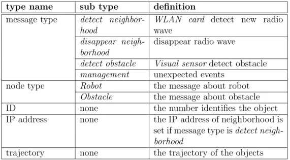
The messages which are managed in this system are three types as follows : Map Manager Message

These messages are sent from Map Manager to Robots through Management Net- work. The details of the contents of this messages are shown Table 5.1.

Robot Management Message

These messages are sent from Robots to Map Manager through Management Net- work. The details of the contents of this messages are shown Table 5.1.

Robot Application Message

These messages are sent from Robots to Robots through Experiment Network. The details of the contents of this messages are shown Table 5.1.

5.2 Application Flows

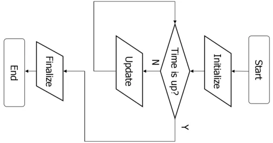
Figure 5.1 describes the flowchart common to the applicationsMap Manager and Robots.

The transactions of these applications can be divided into following simple transactions.

Flowchart of general applications

25

type name sub type definition message type detect neighbor-

hood

WLAN card detect new radio wave

disappear neigh- borhood

disappear radio wave

detect obstacle Visual sensordetect obstacle management unexpected events

node type Robot the message about robot

Obstacle the message about obstacle

ID none the number identifies the object

IP address none the IP address of neighborhood is

set if message type isdetect neigh- borhood

trajectory none the trajectory of the objects

Table 5.1: Map Manager Message type name definition

ID the number identifies the robot

trajectory the trajectory of the objects Table 5.2: Robot Management Message

Initialize

In this phase, Map Manager and Robots initialize their objects and connections through Management Network (see Figure 4.4). At that time Map Manager send the settings (see Table 5.2 more details) to every robot and thereafter start at one time.

Update

These applications are known the time when the system finishes, and if current time is not time up, executesUpdate. This loop phase is divided by short time steps, and in everyUpdatephase they also have similar structure. This transaction is difference between Map Managerand Robot.

Finalize

Finally the applications know the time over, they finalize their objects and finish the applications.

Flowchart of Map Manager

Check updates of environment

26

type name definition

ID the number to identify the robots

priority the priority of the robots trajectory the trajectory of the robots

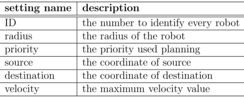
Table 5.3: Robot Application Message setting name description

ID the number to identify every robot

radius the radius of the robot

priority the priority used planning

source the coordinate of source

destination the coordinate of destination velocity the maximum velocity value

Table 5.4: the parameters of setting of robot

Map Manager checks that all of robots detest any hardware messages in current time, for example some robots detect new neighbor robot from the WLAN card or new obstacle from Visual sensorand so on.

Send H/W messages

If the robots detect any emulated hardware messages, Map Manager informs this.

Get messages

Map Manager waits the messages from robots till finishing current step.

Flowchart of Robots

Check updates of environment

The robots check the changes of their environment from the messages from Map Manager and the other robots.

Planning

If the changes of their environment make collision in their trajectory, they start to plan (execute the algorithm Section 3.2). This flow is divided Figure 5.4. The im- plementation of this system, the robots wait constant time and keep on re-planning if they cannot find a trajectory.

Update myself

The robots update their objects, for example the trajectory (if they planned), the WLAN configuration.

27

Initialize

Finalize Time is up?

Update Y

N Start

End

Figure5.1:FlowchartofGeneralApplications

Getmessages

FinallytherobotswaitthemessagesfromMapManagerortheotherrobotstillfinishingcurrentstep.

Inthischapter,themethodwhichemulatesautonomousmobilenetworkedrobotsonPCsisproposedandmentionaboutdetailsofthesemodelingandemulations.

28

Initializ e

Finaliz e Total time is up? Y

N Start

End Get m e ss a g es H/W detect som e thing? Y

N Check upd a te s of environment

Send H/W mes sa g e

Step t ime is up? N

Y

Figure5.2:FlowchartofMapManager

29

Initializ e

Finaliz e Total time is up? Y

N Start

End Get m e ss a g es Detect collision? Y

N Check upd a te s of environment

Planning

Upd a te my se lf

Step t ime is up? N

Y

Figure5.3:FlowchartofRobot

30

Register the trajectory Find a p a th? N

Y Exe cute planner with time t

Create waiting trajectory Start

End

31

Chapter 6 Experiment

In this chapter, how to experiment this system and the definitions of the system environ- ment and emulated descriptions are mentioned. After that the results from this system are shown every different scenario. The experiment which implements the system includes two meanings. First is to evaluate the proposed algorithm. The system enables to con- firm the performance of the algorithm and practicability on real environment. Second are about the system. It make sure whether large-scale mobile networked robots correctly work and communicate each other, the results are compared and evaluated.

6.1 Experiment Definitions

At first the definitions of the experiments every scenarios are defined. The environments are related to the WLAN communication conditions. The definitions of robots set the parameters of the robots. And finally the scenarios define how the robots and obstacles are located and set the destinations.

6.1.1 Emulated Environment Definition

In this paper, the autonomous mobile networked robots are assumed to avoid endangering human life or to reduce cost of repetitive activities. In a disaster or dangerous area, autonomous rescue robots can accomplish various tasks instead of human rescue team.

And in office buildings or homes, autonomous robots assist many kinds of human living, for example it can automatically clean the rooms or hallway. The environment usually classify into indoor and outdoor.

indoor

The WLAN communication conditions of the ”indoor” environment are hard. For example at a office building or home, there exist desks and walls and various obsta- cles interfering communications.

outdoor

32

The ”outdoor” environment enables to communicate easier thanindoorenvironment.

But the WLAN communication conditions of outdoor environment depend on the affections of ”Walls”. If there are many obstacles interfering the communication, the conditions are limited.

The conditions of WLAN communication given above are realized by the configuration values from QOMET. The table 6.1.1 describes the parameters of every environment.

environment α σ

indoor 5.6 2.0

outdoor 3.32 2.0

Table 6.1: the parameters of QOMET

αis the ”path-loss exponent”, andσis used take into account the shadowing component.

From the WLAN emulator QOMET, the connection ranges between robots are calculated as follows :

environment connection range indoor 18.3(m)

outdoor 100.0(m)

Table 6.2: the connection ranges from QOMET

In addition to mentioned hereinbefore, the scenarios describes these whole settings, the number of robots and obstacles and the coordinates of robots and obstacles and of course environments.

6.1.2 Emulated Robot Definition

In this system only the hardware of robots is modeled and simulated. As given previous chapter, these autonomous mobile networked robots rustle in disaster or dangerous area like rescue robots and in office building or home like cleaning or assisting robots. These robots equip motors which move around to accomplish their tasks. These motors are assumed which enable them to turn onmidirectional. And they also have various sensors, a GPS makes them know their absolute coordinate in real time, and a ”Visual sensor”

informs a visual map to them. The autonomous robots of this system equips ”Visual sensor” and detect obstacles around them. The range of this ”Visual sensor” is limited.

The autonomous robots detect the obstacles at first time they are closed to them enough sensing them. These robots communicate each other through WLAN card, this radio wave is sensed by ”Map Manager” on ”Management Network” and after that, robots start to communicate emulated WLAN communication on ”Experiment Network”.

33

parameter value meaning

shape circle the shape of the robot

radius 1.0(m) the radius length of the robot

velocity 0.5(m/sec) the maximum speed of the robot

visual sensor 10.0(m) the visual sensor range

WLAN sensor depending on environment (see previous section)

degree onmidirectional the degree the robots can move

time step 250(msec) the step of execution

Table 6.3: the parameters definition of the robot

The table 6.1.2 describes the parameter definitions of the hardware of autonomous robots of this system.

Basically this system allow various shapes of robots, but both robots and obstacles have a circular shape so that their size can be described by the radius. The system assumes the longest arm of robots, which is the radius of the smallest circle which can cover the object (they have the same center point), the radius of the robots.

The maximum velocity of the robots of this system are set 0.5(m/sec) which is slower than walking velocity of humans.

The range of the ”Visual sensor” equipped can see 10.0(m), this sensor is assumed onmidirectional sensor, for example the camera which the robots equip turn around on- midirection.

WLAN card senses the WLAN communication radio in the range which depend on the environment and the distance between the robots who communicates (see Table 6.1.1).

The system regards the motors of these robots as onmidirectional motors like caterpillar or warm or spider type.

The time step is the limitation of time when Map Manager and Robots execute one main ”Update” phase (see Section 5.2).

6.1.3 Scenario Definitions

In this section, the five Scenarios which is defined the source and destination of every robots and the coordination of obstacles and its size are described. At first as simple case, two Scenario is defined, to confirm the basic flow of this application. Next is more complex Scenario which includes ten 10 robots and 6 obstacles in environment. And finally as large-scale Scenarios are drawn.

Simple Scenarios

The ”Scenario 1” (Table 6.1.3) defines one robot and one obstacle in environment. The initial trajectory of the robot goes through the obstacle.

34

object ID priority radius source destination robot rb01 10 1.0(m) (−20.0,20.0) (20.0,−20.0) obstacle obs01 20 1.0(m) (0.0,0.0) none

Table 6.4: Scenario 1 : One robot and one obstacle

The ”Scenario 2” (Table 6.1.3) defines two robots in environment. The initial trajec- tories also cross each other.

object ID radius source destination robot rb01 1.0(m) (−20.0,20.0) (20.0,−20.0) robot rb02 1.0(m) (20.0,−20.0) (−20.0,20.0)

Table 6.5: Scenario 2 : Two robots

Ten Robots Scenario

This Scenarioplots much complicated both robots and obstacles. It confirms two angles, first is to check the motion-planning method to execute correct. Second are to make them send lots of messages not only Management Networkbut Experiment Network.

Table 6.1.3 and figure 6.1 describes the coordinates of robots and obstacles.

S#1, D#5 S#2, D#10 S#3, D#9

S#4, D#2 S#5, D#7 S#6, D#8

S#7, D#6 S#8, D#1 S#9, D#4 S#10, D#3

(0,0) (15,0) (30,0) (45,0)

(0,15)

(0,30) (15,30) (30,30)

(15,15) (30,15)

Obstacle Src & Dst of robots

Figure 6.1: Scenario 3 : Ten robots and six obstacles

35

object ID radius source destination robot rb01 1.0(m) (0.0,30.0) (15.0,0.0) robot rb02 1.0(m) (15.0,30.0) (0.0,15.0) robot rb03 1.0(m) (30.0,30.0) (45.0,0.0) robot rb04 1.0(m) (0.0,15.0) (30.0,0.0) robot rb05 1.0(m) (15.0,15.0) (0.0,30.0) robot rb06 1.0(m) (30.0,15.0) (0.0,0.0) robot rb07 1.0(m) (0.0,0.0) (30.0,15.0) robot rb08 1.0(m) (15.0,0.0) (30.0,15.0) robot rb09 1.0(m) (30.0,0.0) (30.0,30.0) robot rb10 1.0(m) (45.0,0.0) (15.0,30.0) obstacle obs01 1.0(m) (10.0,10.0) none obstacle obs02 1.0(m) (10.0,20.0) none obstacle obs03 1.0(m) (20.0,10.0) none obstacle obs04 1.0(m) (20.0,20.0) none obstacle obs05 1.0(m) (40.0,10.0) none obstacle obs06 1.0(m) (40.0,20.0) none

Table 6.6: Scenario 3 : Ten robots and six obstacles

Large-Scale Scenario

This large-scale Scenario set fifty and a hundred number of robots. Every coordinate of robots and obstacles are defined by Map Manager at random in the range.

Scenario number of robots number of obstacles initial range

Scenario4 50 20 100(m)

Scenario5 100 40 200(m)

Table 6.7: Scenario 4 and 5 : Fifty and a hundred robots

6.2 Experiment Results

Based on above conditions and definitions, the results of every Scenarioare shown in this section.

6.2.1 Simple Scenarios

Scenario 1 : One robot and one obstacle

Figure 6.2 draws the trajectory of the robot. This Scenario is confirming simply the detection of the obstacle. The robot rb01 starts from its source and approach the Visual

36

sensor range. The robot re-plans its trajectory and avoids the obstacle after detecting it about the coordinate (−8,8).

-20 -10 0 10 20

-30 -20 -10 0 10 20 30

-20 -10 0 10 20

-30 -20 -10 0 10 20 30

-20 -10 0 10 20

-30 -20 -10 0 10 20 30

-20 -10 0 10 20

-30 -20 -10 0 10 20 30

-20 -10 0 10 20

-30 -20 -10 0 10 20 30

obs01 Src rb01

Dst rb01

Figure 6.2: Robot trajectory of Scenario 1 : One robot and one obstacle

Scenario 2 : Two robots

This Scenario also tests another simple detection which the robots receive the WLAN radio wave. Figure 6.3 shows this situation, the robot rb01 and rb02 sense each other about (−8,). As the robot rb01 has lower priority thanrb02 and it re-plans and avoids possible collision.

6.2.2 Scenario 3 : 10 Robots Scenario

ThisScenariois very complicated in small range, ten robots and six obstacles. The radius of robots and obstacles is 1.0(m), the priority is the higher the id of robot is, the more the priority is also.

Figure 6.4 describes Scenario 3 with algorithm 1, and figure 6.5 is algorithm 2’s. The trajectories of algorithm 2 tend to go through linear. At first robot10 goes straight to its destination, and the other robots avoid it depending on the priority (the priority of robot10 is highest). Now from figure 6.5, some interesting results can be shown. For example robot8 go straight till sensing robot10 (about at (22,8) ), but it detects the collision on its trajectory and change it a little. The trajectory of robot3 and robot5 are

37

-20 -10 0 10 20

-30 -20 -10 0 10 20 30

-20 -10 0 10 20

-30 -20 -10 0 10 20 30

-20 -10 0 10 20

-30 -20 -10 0 10 20 30

-20 -10 0 10 20

-30 -20 -10 0 10 20 30

-20 -10 0 10 20

-30 -20 -10 0 10 20 30

-20 -10 0 10 20

-30 -20 -10 0 10 20 30

-20 -10 0 10 20

-30 -20 -10 0 10 20 30

Src rb01

Dst rb01 Src rb02

Dst rb02

-20 -10 0 10 20

-30 -20 -10 0 10 20 30

Src rb01

Dst rb01 Src rb02

Dst rb02

Figure 6.3: Robot trajectories of Scenario 2 : Two robots

same as the situation ofScenario 1, but robot3 did not choose the confusion area, this is why the proposed planning algorithm tends to expand the milestones more free area.

6.2.3 Large Scale Scenario

Following figure 6.6 and 6.7 describes large-scale environments. The radius of robots is 1.0(m) and the obstacle’s is at random from 1.0(m) to 2.0(m). Accurate numbers of the robots are fifty-five and a hundred and ten. The lines are the trajectory of each robot, and + is the coordinate of the obstacles. These figures show collision avoidance which every robot does not cross with obstacles.

In this chapter, the definitions of the experiment environments and the Scenarioevery situation (simple and complicated and large-scale) are defined. Finally the results every Scenarioare described.

38