One Dimensional Viscous Conservation Laws with Discontinuous Initial Data(Mathematical Analysis in Fluid and Gas Dynamics)

One

Dimensional Viscous

Conservation

Laws with

Discontinuous Initial

Data

Harumi

Hattori

Department

of Mathematics

West

Virginia

University

Morgantown,

WV

26506-6310

[email protected]

1

Introduction

I summarize the results concerning the existence and the decay rates obtained for the

viscous conservation laws with discontinuous initial data. An interesting case is the

hyperbolic-parabolic case where the system contains both hyperbolic equations and

parabolic equations.

What

we

consider is the initial value problem where there is

a

discontinuity in the

initial data at $x=0$. It is well-known that the discontinuities in the initial data persist

along$x=0$for$t>0$

.

Tostudythedecayratesweusethe Laplaceand inversetransforms

to obtainthe solution representations,which involve the Green functions. We first apply

theLaplacetransform toobtainasystemofordinary differentialequationsfor$x>0$and

$x<0$

.

Weusethe Rankine-Hugoniot conditions as the boundary conditionsto solve the

system ofordinarydifferential equations. Then, theinverseLaplacetransformis applied

to obtain the solutionrepresentations, fromwhichweobtain the existence andthe decay

rates of solutions.

There are

numerous

results for the viscous conservation laws with smooth initial

data. On the other hand, there are only a few results with discontinuous initial data.

Hoff [1, 2, 3, 4, 5] studied the compressible Navier-Stokes equations. Hoff and Khodja

[6] and Pego [17] discussedthe nonmonotonecase. UsingtheGreen’s functions to study

the existence, stability,

or

decay rates of solutions is widely practiced. Kawashima

$[7, 8]$ studied the large time behavior of hyperbolic-parabolic equations. Nishihara [15]

studied the

wave

equations with damping. Nishihara, Wang, andYang [16] studied the

$L^{\mathrm{p}}$-convergence ratefor the p-system with damping. The decay ratesof

smoothsolutions

to travelingwavesolutionsor diffusionwaves for hyperbolic-parabolic conservationlaws

have been discussed in various literature. Liu and Zeng $[10, 11]$ and Zeng [18] discussed

the decay rates ofsolutions to the diffusion

waves.

Liu [9] also studied the decay rates

ofsolutions to the traveling

wave

solutions. The solutions

are

represented through the

Fouriertransform. Zumbrun and Howard $[20, 21]$ and Mascia and Zumbrun [12, 13, 14]

This paper consists of four sections. In Section 2

we

describe the problem and the

solution representations are obtained in Section 3. The existence and decay results

are

stated in Section 4. Remarks about the results and some future problems are given in

Section 5.

2

Description of the

problem

Thesystem weconsider is given by

$v_{t}-u_{x}$

$u_{t}-f(v)_{x}$

$=0$,

$=u_{xx}$, (2.1)

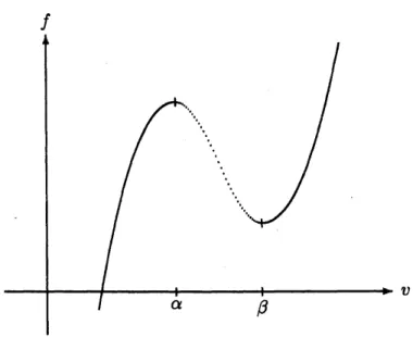
where $f,$ $v$, and$u$

are

the stress, strain, and velocity, respectively. We

assume

that $f$ is

asmooth function of$v$. $f$

can

be monotone

or

nonmonotone. Inthe nonmonotone

case

the graph of$f$ is given in Fig. 1.1.

Figure 1.1: Graphofa nonmonotone stress strain relation.

The initial data

are

given by

$(v,u)(x, 0)=(v_{0},u_{0})(x)=\{$

$(v_{\mathrm{t}}, u_{1})(x)$, $x<0$,

$(v_{r}, u_{\mathrm{r}})(x),$ $x>0$, (2.2)

wherethere isa discontinuity at $x=0$

.

We

assume

that theinitial datasatisfy that

$C_{0}= \sup_{1\leq \mathrm{P}\leq\infty}||v_{0}-\overline{v},$

is finite, where$p_{0}$ is

a

constant largerthan

or

equal to two, $\underline{L}^{p}$ is the piecewise $L^{\mathrm{p}}$

norm

in space given by

$||v||_{\underline{L}^{\mathrm{p}}}=( \int_{x<0}v(x, t)^{p}dx)^{1/\mathrm{p}}+(\int_{x>0}v(x, t)^{p}dx)^{1/p}=||v||_{L_{-}^{\mathrm{p}}}+||v||_{L_{+}^{\mathrm{p}}}$,

and$(\overline{v},\overline{u})$

are

piecewiseconstant statessuch that$\overline{v}$is thepiecewiseconstant straingiven

by

$\overline{v}=\{$

$\overline{v}_{-}$, $x<0$, $\overline{v}_{+}$, $x>0$

(2.4) and $\overline{u}$ is a constant velocity. In the nonmonotone case,

we

choose

$\overline{v}_{-}\in(0, \alpha]$ and $\overline{v}_{+}\in[\beta, \infty)$ so that $f(\overline{v}_{-})=f(\overline{v}_{+})$ is satisfied. In the hyperbolic case, we need to

assume

$\overline{v}_{-}=\overline{v}_{+}$

.

One important difference is that in the

case

of monotone $f$, the

strength of discontinuity decays exponentially while in the

case

of nonmonotone $f$, it

does not and it is not small by any

means.

It is well known that the discontinuity in

$v$ persists for $t>0$ along $x=0$ whether

we

deal with nonmonotone $f$ or monotone $f$

$(f’>0)$ while $u$becomes continuous for $t>0$

.

The Rankine-Hugoniot condition along

$x=0$ is given by

$u(0_{+}, t)$ $=$ $u(\mathrm{O}_{-}, t)$,

$-f(v(0_{+}, t))+f(v(0_{-}, t))$ $=$ $u_{x}(0_{+}, t)-u_{x}(0_{-}, t)$

.

(2.5)

3

Solution

representations

Substituting $(v_{\pm}, u_{\pm})=(w_{\pm}+\overline{v}_{\pm}, z_{\pm}+\overline{u})$ in (2.1) and applying the Laplacetransform,

we

obtain the systems of ordinary differential equations for $x>0$ and $x<0$

.

Then,

solvingtheordinary differentialequationswiththe Rankine-Hugoniot condition (2.5)

as

the boundary conditions at $x=0$ and applying the inverse transforms, we obtain the

following solution representations.

$=w_{+}(x,t)f’( \overline{v}_{-})\int_{-\infty}^{0}T_{30}^{2-}(x,\eta,t)w(\eta,0)d\eta-\int_{-\infty}^{0}T_{20}^{2-}(x,\eta, t)z(\eta,0)d\eta$

$+ \int_{0}^{t}\int_{-\infty}^{0}T_{31}^{2-}(x, \eta, t-s)\tilde{g}_{2}(\eta, s)d\eta ds$

$+f’( \overline{v}_{+})\int_{0}^{\infty}R_{30}^{+}(x,\eta, t)w(\eta, 0)d\eta+\int_{0}^{\infty}R_{20}^{+}(x,\eta, t)z(\eta,\mathrm{O})d\eta$ $+ \int_{0}^{t}\int_{0}^{\infty}R_{31}^{+}(x,\eta, t-s)\tilde{g}_{2}(\eta, s)d\eta ds$

$+ \mathrm{e}^{-f’(\overline{v}_{+)t}}w_{0}(x)-\int_{0}^{t}e^{-f’(\overline{v}_{+})(t-*)}\tilde{g}_{2}(x, s)ds$

$+f’( \overline{v}_{+})\int_{0}^{x}P_{30}^{+}(x-\eta,t)w(\eta, \mathrm{O})d\eta-\int_{0}^{x}P_{20}^{+}(x-\eta,t)z(\eta,\mathrm{O})d\eta$

$+f’( \overline{v}_{+})\int_{x}^{\infty}P_{30}^{+}(\eta-x, t)w(\eta, 0)d\eta+\int_{x}^{\infty}P_{20}^{+}(\eta-x, t)z(\eta, \mathrm{O})d\eta$ $+ \int_{0}^{t}\int_{x}^{\infty}P_{31}^{+}(\eta-x, t-s)\tilde{g}_{2}(\eta, s)d\eta ds$,

$z_{+}(x, t)$

$=$ $-f’( \overline{v}_{-})\int_{-\infty}^{0}T_{20}^{1-}(x, \eta, t)w(\eta, 0)d\eta+\int_{-\infty}^{0}T_{10}^{1-}(x, \eta,t)z(\eta, 0)d\eta$

$- \int_{0}^{t}\int_{-\infty}^{0}T_{21}^{1-}(x, \eta, t-s)\tilde{g}_{2}(\eta, s)d\eta ds$

$-f’( \overline{v}_{+})\int_{0}^{\infty}R_{20}^{+}(x+\eta, t)w(\eta, \mathrm{O})d\eta-\int_{0}^{\infty}R_{10}^{+}(x+\eta,t)z(\eta, \mathrm{O})d\eta$ $- \int_{0}^{t}\int_{0}^{\infty}R_{21}^{+}(x+\eta, t-s)\tilde{g}_{2}(\eta, s)d\eta ds$

$-f’( \overline{v}_{+})\int_{0}^{x}P_{20}^{+}(x-\eta, t)w(\eta, 0)d\eta+\int_{0}^{x}P_{10}^{+}(x-\eta, t)z(\eta, \mathrm{O})d\eta$

$- \int_{0}^{t}\int_{0}^{x}P_{21}^{+}(x-\eta, t-s)\tilde{g}_{2}(\eta, s)d\eta ds$

$+f’( \overline{v}_{+})\int_{x}^{\infty}P_{20}^{+}(\eta-x, t)w(\eta, 0)d\eta+\int_{x}^{\infty}P_{10}^{+}(\eta-x, t)z(\eta, \mathrm{O})d\eta$

$+ \int_{0}^{t}\int_{x}^{\infty}P_{21}^{+}(\eta-x, t-s)\tilde{g}_{2}(\eta, s)d\eta ds$, (3.1)

where $\overline{g}_{2}(w_{\pm})=[f(\overline{v}_{\pm}+w_{\pm})-f(\overline{v}_{\pm})-f’(\overline{v}_{\pm})w_{\pm}]$. The similar expressions can be

ob-tained for $w$-and $z_{-}$

.

Here, the subscripts $+\mathrm{a}\mathrm{n}\mathrm{d}$ –stand for $x>0$ and $x<0$,

respectively. Differentiating$w_{+}$ and $z_{+}$ in $x$ and performing theintegration by parts in

$\eta$,

we

obtain

as

the representation for the derivatives

$w_{+x}(x, t)$

$=$ $f’(\overline{v}_{+})(w_{0}(0_{+})-w_{0}(0_{-}))T_{30}^{3-}(x, 0, t)-(z(\mathrm{O}_{-}, 0)-z(0_{+}, 0))T_{20}^{3-}(x, 0, t)$

$+ \int_{0}^{t}T_{31}^{3-}(x, 0, t-s)\{\tilde{g}_{2}(w(0_{+}, s))-\tilde{g}_{2}(w(0_{-}, s)\}ds$

$+\mathrm{s}\mathrm{i}\mathrm{m}\mathrm{i}\mathrm{l}\mathrm{a}\mathrm{r}$ terms

as

in _{$w_{+}(x, t)$},

$z_{+x}(x, t)$

$=$ $(z(0_{+}, 0)-z(0_{-}, 0))T_{10}^{2-}(x, 0, t)+f’(\overline{v}_{+})(w(0_{-}, 0)-w(0_{+}, 0))T_{20}^{2-}(x, 0, t)$

$+ \int_{0}^{t}T_{21}^{2-}(x,0, t-s)\{\tilde{g}_{2}(w(0_{-}, s))-\tilde{g}_{2}(w(0_{+}, s))\}ds$

$+\mathrm{s}\mathrm{i}\mathrm{m}\mathrm{i}\mathrm{l}\mathrm{a}\mathrm{r}$ terms

as

in _{$z_{+}(x, t)$}. (3.2)

In the above expressions

$R_{mn}^{\pm}(x, \eta, t)=\frac{1}{2\pi i}\int_{\Gamma}\frac{(\tilde{\mu}_{\pm}-\tilde{\mu}_{\mp})}{2(\tilde{\mu}_{+}+\tilde{\mu}-)}\tilde{\mu}_{\pm}^{m}\lambda^{n}e^{\lambda\{t\mp\overline{\mu}\pm(x+\eta)\}}d\lambda$ ,

$P_{mn}^{\pm}(x- \eta, t)=\frac{1}{2\pi i}\int_{\Gamma}\frac{1}{2}\tilde{\mu}_{\pm}^{m}\lambda^{n}e^{\lambda\{t-\overline{\mu}\pm(x-\eta)\}}d\lambda$,

where $\tilde{\mu}_{\pm}=\sqrt{\epsilon\lambda+f’(\overline{v}\pm)}^{1}$ and

$\Gamma$ is a path in the complex A-plane. $T_{mn}^{l\pm}$ and $R_{mn}^{\pm}$ account

for the transmission and reflection, respectively. $P_{mn}^{\pm}$ is basically the same asthe usual

Green’s function.

4

Existence and decay

estimates

After performingthe integrations in A for$\tau_{mn}^{\iota\pm},$ $R_{mn}^{\pm}$, and $P_{mn}^{\pm}$, weobtain the following

estimates.

Lemma 4.1 For$n=0$ and$m=1$ or$n=1,$ $T_{mn}^{l\pm},$ $R_{mn}^{\pm}$, and $P_{mn}^{\pm}$ satisfy the estimates

$|T_{mn}^{l\pm}(x, \eta, t)|$

$=O(1)t^{-\frac{n+1}{2}}e^{-K\frac{(t-\ovalbox{\tt\small REJECT}_{J’(\varpi_{\mp})}^{x}-\ovalbox{\tt\small REJECT} f’(\emptyset\pm))^{2}}{t}}+O(1)t^{-\frac{n+1}{2}}e^{-\kappa^{\llcorner\llcorner^{2}}}x-\Delta\iota+\mathcal{R}$

, $|R_{mn}^{\pm}(x+\eta, t)|$ $=O(1)t^{-\oplus}e^{-K\frac{(t-\mu_{v}x+f(\pm)\rangle^{2}}{\mathrm{t}}}’+O(1)t^{-\frac{\mathfrak{n}\neq 1}{2}}e^{-K^{x}}t+Rrightarrow+\mathit{1}_{-}^{2}$ , $|P_{mn}^{\pm}(x-\eta, t)|$ $=$ $o(1)t^{-\frac{\mathfrak{n}+1}{2}}e^{-K\frac{(t-\mu_{\mathrm{t}\emptyset\pm)}x-)^{2}J’}{t}}+O(1)t^{-\frac{n\neq 1}{2}}e^{-K^{\llcorner\sim-}}+\mathcal{R}\Delta_{\iota}\mathrm{L}^{2}$ ,

where $K$ is apositive constant and$\mathcal{R}$ represents residual $te7ms$ decaying

faster

than the

first

two terms.

For$T_{mn}^{l\pm}$,

if

$n=0$ and$m=2$, using the convolution theorem, we obtain

$|T_{mn}^{i\pm}(x, \eta, t)|$ $=$ $| \frac{1}{2\pi i}\int_{\Gamma}\tilde{\mu}_{\pm}\frac{\tilde{\mu}_{\mp}^{l}}{\tilde{\mu}_{\pm}^{l-1}(\tilde{\mu}_{+}+\tilde{\mu}-)}\tilde{\mu}_{\pm}e^{\lambda t\pm\mu\mp^{x\mp\mu\pm\eta}}d\lambda|$

$\leq$ $o(1) \int_{0}^{t}(t-s)^{-1}2e^{-f’(\overline{v})(t-*)}+|T_{10}^{l\pm}(x, \eta, s)|ds$. (4.1)

Similarly,

_if

$n=0$ and$m=3$,

$|T_{mn}^{l\pm}(x, \eta, t)|$ _$=$ $| \frac{1}{2\pi i}\int_{\Gamma}\tilde{\mu}_{\pm}^{2}\frac{\tilde{\mu}_{\mp}^{l}}{\tilde{\mu}_{\pm}^{l-1}(\tilde{\mu}_{+}+\tilde{\mu}_{-})}\tilde{\mu}_{\pm}e^{\lambda t\pm\mu\mp^{x\mp\mu\pm\eta}}d\lambda|$

$\leq$ $o(1) \int_{0}^{t}e^{-J’(\overline{v}}+)(t-*)|T_{10}^{l\pm}(x, \eta, s)|ds$. (4.2)

Similar estimates

can

be obtained

_for

$R_{mn}^{\pm}$, and$P_{mn}^{\pm}$

.

Using the solution representationsobtained in the previous section, weconstruct an

iteration scheme in the Banach space $X$ with the norm given by

$||(v,u)(\cdot, t)||_{X}$ $=$ $\sup$ $\{(t+1)^{\tau_{\dot{\mathrm{p}}^{-}2}^{11}}||(v-\overline{v},u-\overline{u})(\cdot,t)||_{L^{\mathrm{p}}}$

$1\leq \mathrm{P}\leq\infty,1\leq q\leq \mathrm{P}0,0\leq t<\infty$

The iteration can be constructed by putting upper-subscripts $(k+1)$ _to the variables

on the left hand sides and $(k)$ to those on the right hand sides in (3.1), (3.2), and etc.

After estimating the terms in thesolution representationswith the helpof Lemma 4.1,

we

obtain

Lemma 4.2 Let

$N^{(k)}(t)$ $=$ _$\sup$ $\{||w^{(k)},$$z^{(k)}||_{L^{\mathrm{p}}}(1+\tau)^{\iota}\mathrm{z}^{-\frac{1}{2p}}$

$1\leq P\leq\infty,1\leq q\leq P\mathit{0},0\leq r<t$

$+||w_{x}^{(k)},$ $z_{\pm x}^{(k)}-(z(0_{+}, \mathrm{O})-z(\mathrm{O}_{-}, 0))T_{10}^{2\mp}(x, 0, t)||_{\mathrm{A}^{q}}(1+\tau)^{l^{-}T_{l}}\}11$.

Then, the following inequality

$N^{(k+1)}(t)\leq C_{1}C_{0}+C_{2}C_{3}N^{(k)}(t)^{2}$

hol&, where $C_{0}$ is the constant

defined

in $($2.$S),$ $C_{1}$ and $C_{2}$

are

positive constants

from

the Green’sfunctions, and $C_{3}= \max_{|w|\leq 1}|f’’(\overline{v}_{+}+w)|$

.

IFbom the above lemmaand the contraction mapping, we

can

easily obtain

Theorem 4.3 There exists a constant$\overline{C}_{0}$ such that

if

the initial data satisfy $C_{0}\leq\overline{C}_{0}$,

where $C_{0}$ is given in (2.3), the global solutions exist in $X$ and satisfy the decay rates

given by

$||v-\overline{v},$ $u-\overline{u}||_{L^{p}}$ $=$ $o(1)(t+1)^{-\frac{1}{2}++_{p}},$ $1\leq p\leq\infty$,

$||v_{x},$_{$u_{\pm x}-(u_{0}(0_{+})-u_{0}(0_{-}))T_{10}^{2\mp}(x, 0, t)||_{\underline{L}^{\mathrm{p}}}$ $=$} $O(1)(t+1)^{-\frac{1}{2}+_{2p}}\perp,$ _{$1\leq p\leq p0$},

where $T_{10}^{2\mp}(x, 0, t)$ are

diffusion

waves singular at $t=0$

.

Also, the Rankine-Hugoniot

condition is

_satisfied

across

$x=0$.

5

Concluding remarks

In this concluding section we discuss

some

observations and the possible future work.

The discontinuity in the initial data brings various interesting differences between the

hyperbolic variable $v$ and the parabolic variable $u$

.

They

are

summarized as follows.

(1) The first two terms on the right hand side of each expression in $w_{+x}(x,t)$ and

$z_{+x}(x, t)$ are from the discontinuity in the initial data. They

are

diffusion waves. $T_{10}^{2-}$

behaves like a heat kernel approaching

a

delta function

as

$t\downarrow \mathrm{O}$

.

On the other hand,

$T_{20}^{2-},$ $T_{20}^{3-}$, and $T_{30}^{3-}$ are not singular

as

$t\downarrow \mathrm{O}$

.

The parabolic variable has

a

singularity

in the derivative which behaves like aheat kernel. This captures the way the parabolic

variable becomes continuous for $t>0$. On the other hand the hyperbolic variable

remains discontinuous. Therefore, there inno singular wave in the derivative.

(2)The maineffect

near

$t=0$_{is given by the exponentially decaying term}$e^{-f’(\varpi_{+})t}w_{0}(x)$

for thehyperbolic variable and the diffusive terms $\int_{0}^{x}P_{10}^{+}(x-\eta, t)z(\eta, 0)d\eta+\int_{x}^{\infty}P_{10}^{+}(\eta-$

(3) $m$and$n$ forthe hyperbolicvariableand the parabolic variablearedifferent. This

affects the behavior ofthesevariables especially near $t=0$

.

The result obtained should be extended for the following prototype systems. First,

in the Lagrangiancoordinates, the viscosity terms

are

nonlinear as shownbelow.

$v_{t}-u_{x}$ $=0$,

$u_{t}-f(v)_{x}$ $=$ $( \epsilon\frac{u_{x}}{v})_{x}$,

It is important to discuss the changes necessary to treat the nonlinear nature of the

viscous term. Also, it is interestingto extend the result to the nonisothermal

case

with

various viscosity terms. Another interesting problem is to extend to the initial data

with different values at $x=\pm\infty$. This will include the Riemann problems for viscous

conservationlaws. The difficulty isthe factthat the solutions will not approachpiecewise

constant states. We need to find the approximate solutions to which the solutions will

approach.

References

[1] D. Hoff, Construction of solutions for compressible, isentropic Navier-Stokes

equa-tions in

one

space dimension with nonsmooth initialdata, Proceedings of theRoyal

Society of Edinburgh, 103A (1986), 301-315.

[2] D. Hoff, Discontinuous solutions of the Navier-Stokes equations for compressible

flow, Arch. Rational Mech. Anal. 114 (1991), 15-46.

[3] D. Hoff, Global well-posedness ofthe Cauchy problem for the Navier-Stokes

equa-tionsofnonisentropic flow with discontinuous initial data. J. DifferentialEquations

95 (1992),

33-74.

[4] D. Hoff, Global solutions of the Navier-Stokes equations for multidimensional

com-pressible flow with discontinuous initial data. J. Differential Equations 120 (1995),

215-254.

[5] D. Hoff, Discontinuous solutions of theNavier-Stokesequationsfor multidimensional

flows ofheat-conducting fluids. Arch. Rational Mech. Anal. 139 (1997),

303-354.

[6] D. Hoff and M. Khodja, Stability of coexisting phases for compressible van der

Waals fluids. SIAM J. Appl. Math. 53 (1993), 1-14.

[7] S. Kawashima, Systems ofahyperbolic-parabolic composite type withapplications

to the equations ofmagnetohydrodynamics. Ph.D. Thesis, Kyoto University, 1983.

[8] S. Kawashima, Large-timebehaviour of solutions tohyperbolic-parabolic systemsof

conservation laws and applications. Proc. Roy. Soc. Edinburgh Sect. A 106 (1987),

[9] T.P. Liu, Pointwise convergence to shock waves for viscous conservation laws.

Comm. Pure Appl. Math. 50 (1997), 1113-1182.

[10] T.P. Liu and Y. Zeng, Large time behavior of solutions of general quasilinear

hyperbolic-parabolic systems of conservation laws. Mem. Amer. Math. Soc. 125,

(1997).

[11] T.P. Liu and Y. Zeng, Compressible Navier-Stokes equations with zero heat

con-ductivity. J. Differential Equations 153 (1999), 225-291.

[12] C. Mascia and K. Zumbrun, Pointwise Greenfunction bounds for shock profiles of

systemswith real viscosity. Arch. Ration. Mech. Anal. 169 (2003), 177-263.

[13] C. Mascia and K. Zumbrun,Stabilityofsmall-amplitudeshockprofiles of symmetric

hyperbolic-parabolic systems. Comm. Pure Appl. Math. 57 (2004), 841-876.

[14] C. Mascia and K. Zumbrun, Stability of large-amplitude viscous shock profiles of

hyperbolic-parabolic systems. Arch. Ration. Mech. Anal. 172 (2004), 93-131.

[15] K. Nishihara, $IP- L^{q}$ estimates of solutions to the damped

wave

equation in

3-dimensional space and their application. Math. Z. 244 (2003), 631-649.

[16] K. Nishihara, W. Wang, and T. Yang, $I\nearrow$-convergence rate to nonlinear diffusion

waves

forp–system with damping. J. Differential Equations 161 (2000), 191-218.

[17] R.L. Pego, Phase transitions in one-dimensional nonlinear viscoelasticity:

admissi-bility and stability, Arch. Rat. Mech. Anal. 97 (1987),

353-394.

[18] Y. Zeng, $L^{1}$ asymptotic behavior of compressible, isentropic, viscous 1-D flow.

Comm. Pure Appl. Math. 47 (1994), 1053-1082.

[19] K. Zumbrun, Dynamical stabilityof phasetransitions in the p–system with

viscosity-capillarity. SIAM J. Appl. Math. 60 (2000), 1913-1924

[20] K. Zumbrun and P. Howard, pointwise semigroup methods andstability of viscous

shock

waves.

Indiana Univ. Math. J. 47 (1998), 741-871.

[21] K. Zumbrun and P.Howard,Erratato: “_{Pointwisesemigroup methods,} and stability

of viscous shockwaves” [Indiana Univ. Math. J. 47 (1998), 741-871]. IndianaUniv.