精度保証付き数値計算による楕円型作用素の逆作用素ノルム評価 (新時代の科学技術を牽引する数値解析学)

精度保証付き数値計算による楕円型作用素の

逆作用素ノルム評価

$\ovalbox{\tt\small REJECT}^{\backslash }$部善

(Yoshitaka Watanabe)*

九州大学情報基盤研究開発センター

(ResearchInstitute for InformationTechnology, Kyushu University)

独立行政法人科学技術振興機構，CREST

(CREST, Japan Scienceand Technology Agency) Abstract

本稿では，2 階楕円型線形作用素に対する可逆性と逆作用素ノルムの上界値を数学的に厳密な意味で

保証する数値計算法をいくつか紹介する．

1

Introduction

Let $\Omega\subset \mathbb{R}^{d}$

be a bounded polygonal or polyhedral domain $(d=1,2,3)$, and for some integer $m$, let

$H^{m}(\Omega)$ denote the complex$L^{2}$

-Sobolev space of order $m$on$\Omega$.

We define the Hilbert space

$H_{0}^{1}(\Omega):=\{u(x)\in H^{1}(\Omega)|u(x)=0, x\in\partial\Omega\}$

with the inner product $(\nabla u, \nabla v)_{L^{2}(\Omega)}$ and thenorm $\Vert u\Vert_{H_{0}^{1}(\Omega)}$ $:=\Vert\nabla u\Vert_{L^{2}(\Omega)}$, where $(u, v)_{L^{2}(\Omega)}$ implies

$L^{2}$-inner producton$\Omega$

.

Let

$H(\Delta;L^{2}(\Omega)):=\{u(x)\in H_{0}^{1}(\Omega)|\triangle u\in L^{2}(\Omega)\}$

be a Banach space with respect to the graph norm $\Vert u\Vert_{L^{2}(\Omega)}+\Vert\Delta u\Vert_{L^{2}(\Omega)}$. Since $\Omega$ is in a class of

the bounded domain with a Lipschitz continuous boundary, the embedding $H(\triangle;L^{2}(\Omega))\mapsto H_{0}^{1}(\Omega)$ is

compactby theRellich compactnesstheorem.

Considerthe linear elliptic operator

$\mathscr{L}u:=-\Delta u+b\cdot\nabla u+cu$ ₍₁₎

for $b\in L^{\infty}(\Omega)^{d},$ $c\in L^{\infty}(\Omega)$ with norms

$\Vert b\Vert_{L(\Omega)^{d}}\infty=ess\sup_{x\in\Omega}\sqrt{|b_{1}(x)|^{2}++|b_{d}(x)|^{2}}, \Vert c\Vert_{L(\Omega)}\infty=ess\sup_{x\in\Omega}|c(x)|,$

respectively.

The aim of this paper is to proposesomeprocedures for verifying the invertibilityofan $\mathscr{L}$ with a

computableupper bound$M>0$ satisfying

$\Vert u\Vert_{H_{o}^{1}(\Omega)}\leq M\Vert \mathscr{L}u\Vert_{H(\Omega)}-1, \forall u\in H_{0}^{1}(\Omega)$ (2)

or

$\Vert u\Vert_{H_{0}^{1}(\Omega)}\leq M\Vert \mathscr{L}u\Vert_{L^{2}(\Omega)}, \forall u\in H(\triangle;L^{2}(\Omega))$ (3)

or

$\Vert\triangle u\Vert_{L^{2}(\Omega)}\leq M\Vert \mathscr{L}u\Vert_{L^{2}(\Omega)}, \forall u\in H(\triangle;L^{2}(\Omega))$. (4)

*This is a joint work with Takehiko Kinoshita (Kyoto University) and Mitsuhiro T. Nakao (National Institute of

For example, whenonetryto find$u\in H_{0}^{1}(\Omega)$ (weak sense) satisfying nonlinear_problems

$-\triangle u(x)=f(x, u, \nabla u) , x\in\Omega$ ₍₅₎

with certain propertiesfor$f$ and apply infinite-dimensional verification approach for$u$, the norm

esti-mations (2), (3), (4) are required [13, 16, 18, 19, 20]. We note that the upper bound $M$ can also be

appliedto verified computationsofeigenvalueexclosures in Hilbert spaces [25].

2

Approximation subspace and

notations

Let $S_{h}$ be a finite dimensional approximation subspace of $H_{0}^{1}(\Omega)$ dependent on the parameter _$h>$ O. For example, $S_{h}$ is taken to be afiniteelement subspace with mesh size $h$

.

Let $P_{h}$ :$H_{0}^{1}(\Omega)arrow S_{h}$ denote

the $H_{0}^{1}$-projection definedby

$(\nabla(\phi-P_{h}\phi), \nabla v)_{L^{2}(\Omega)}=0, \forall v\in S_{h}$, ₍₆₎

and suppose that $P_{h}$ has the following approximation properties.

$\Vert v-P_{h}v\Vert_{H_{0}^{1}(\Omega)}\leq C(h)\Vert\triangle v\Vert_{L^{2}(\Omega)}, \forall v\in H(\triangle;L^{2}(\Omega))$, (7)

$\Vert v-P_{h}v\Vert_{L^{2}(\Omega)}\leq C(h)\Vert v-P_{h}v\Vert_{H_{0}^{1}(\Omega)}, \forall v\in H_{0}^{1}(\Omega)$, (S)

where $C(h)>0$isapositiveconstantwhich is numericallydeterminedwith the propertythat$C(h)arrow 0$

as $harrow 0$_{. We emphasize that especially the estimate (7) is indispensable in our argument and the}

compactness of the embedding $H(\triangle;L^{2}(\Omega))\mapsto H^{1}(\Omega)$ is essential in getting the _{constant $C(h)$ with}

desired property. Usually the second estimation (8) for $P_{h}$ is derived by using a technique so called

Aubin-Nitsche’strick [1].

These assumptions (7) and (8) hold formanyfinite element subspaces of$H_{0}^{1}(\Omega)[1$, 9, 10, 11, 12, 15$]$or

function spaces of Fourier serieswith finitetruncation [23]. For example it canbe takenas $C(h)=h/\pi$

and $h/(2\pi)$ for bilinear and biquadratic element, respectively, for the rectangular mesh on the square

domain [9], and $C(h)=0.493h$ _{for the linear and uniform} triangular mesh of the convex polygonal

domain [3, 6]. Furthermore, a constructive apriori $L^{\infty}$ error

estimate for the projection $P_{h}$ can also

be obtained [7, 8]. In case of

nonconvex

polygonal domain, there are some useful techniques and

consideration to obtain mathematicallyrigorousupper bounds forthe constant$C(h)$ _{satisfying (7) with}

adequate orderforsuch nonconvexdomains [2, 5, 14, 26, 27, 28].

Define basis functionof$S_{h}$ by $\{\phi_{i}\}_{i=1}^{N}$ for_{$N:=\dim S_{h}$} and$N\cross N$ _matrices$G,$$D,$ $L$, andHermitian

matrix $E$by

$[G]_{ij}=(\nabla\phi_{j}, \nabla\phi_{i})_{L^{2}(\Omega)}+(b\cdot\nabla\phi_{j}+c\phi_{j}, \phi_{i})_{L^{2}(\Omega)}$, (9)

$[D]_{ij}=(\nabla\phi_{j}, \nabla\phi_{i})_{L^{2}(\Omega)}$, ₍₁₀₎

$[L]_{ij}=(\phi_{j}, \phi_{i})_{L^{2}(\Omega)}$, (11)

$[E]_{ij}=(b\cdot\nabla\phi_{j}+c\phi_{j}, b\cdot\nabla\phi_{i}+c\phi_{i})_{L^{2}(\Omega)}$, (12)

respectively. Since $D$ and $L$ are positive definite, they can _{be decomposed} as _{$D=D^{1/2}D^{H/2}$ and}

$L=L^{1/2}L^{H/2}$ _where $H$ indicates the conjugate _{transposition. Usually} $D^{1/2}$ _and $L^{1/2}$ are _{the lower}

triangularmatrices. We assumethat$G$has theinverse and let_{$C_{p}>0$denote the Poincar\’e}

or Rayleigh-Ritz constants whichsatisfies

$\Vert u\Vert_{L^{2}(\Omega)}\leq C_{p}\Vert\nabla u\Vert_{L^{2}(\Omega)}, u\in H_{0}^{1}(\Omega)$. (13)

3

Estimation

(2)

This section is devoted to an upperbound $M$_safisfying

with theinvertibilityof$\mathscr{L}.$

It is well-known that for each$\xi\in H^{-1}(\Omega)$ there exists aunique$\psi\in H_{0}^{1}(\Omega)$ satisfying

$\{\begin{array}{ll}-\Delta\psi = \xi in \Omega,\psi = 0 on \partial\Omega.\end{array}$

becomes

$(\triangle;L(\Omega))\mapsto Byd$

compact because $\psi be1$ongs t$oH(\triangle;L^{2}(\Omega))andthee$_{mbedding H}

efine t$hism$apping $\xi\mapsto\psi by(-\Delta)^{-1}:H^{-1}(\Omega)arrow H_{0}^{1}(\Omega),$

$amap(-\Delta)^{-1}|_{L^{2}(\Omega}4^{:L^{2}(\Omega)}arrow H_{0}^{1}(\Omega)H^{1}(\Omega)is$

compact. Wedefine alinear compact operator$F:H_{0}^{1}(\Omega)arrow H_{0}^{1}(\Omega)$ by

$Fu:=(-\Delta)^{-1}|_{L^{2}(\Omega)}(-b\cdot\nabla u-cu)$

.

₍₁₄₎ Then since the term $-b\cdot\nabla u-cu$ maps each bounded set of $H_{0}^{1}(\Omega)$ to abounded set of $L^{2}(\Omega)$, the

operator$F$ becomes compact

on

$H_{0}^{1}(\Omega)$, and the following is true. Lemma 1. [13, Theorem 2.3]

If $I-F$

on

$H_{0}^{1}(\Omega)$ is invertible then

so

is$\mathscr{L}$, and $M>0$

of (2) canbe taken

as

satisfying

$\Vert(I-F)^{-1}u\Vert_{H_{0}^{1}(\Omega)}\leq M\Vert u\Vert_{H_{0}^{1}(\Omega)}, \forall u\in H_{0}^{1}(\Omega)$

.

(15)

3.1

1st

estimation

of (2)

Our first result for (2) is asfollows.

Theorem 1. [17, Theorem 1] For

$C_{1}:=\Vert b\Vert_{L^{\infty}(\Omega)^{d}}+C_{p}\Vert c\Vert_{L\infty(\Omega)}$, (16)

if$C_{p}C_{1}<1$then $I-F$ isinvertible and $M$ of₍₂₎ can_{be taken}

as

$M= \frac{1}{1-C_{p}C_{1}}$

.

(17)

3.2

2nd

estimation

of (2)

We define

$C_{2} :=\Vert b\Vert_{L\infty(\Omega)^{d}}+C(h)\Vert c\Vert_{L\infty(\Omega)}$, (18)

$K:=\{\begin{array}{ll}C(h)(C_{p}\Vert\nabla\cdot b\Vert_{L\infty(\Omega)}+C_{1}) , if b\in W^{1,\infty}(\Omega)^{d},C_{r}C_{2}, if b\in L^{\infty}(\Omega)^{d},\end{array}$ (19)

$\rho:=\Vert D^{T/2}G^{-1}D^{1/2}\Vert_{2}$, (20)

where $\Vert\cdot\Vert_{2}$ standsfor matrix 2-norm. Notethat

$\rho$can be represented by $\rho^{-1}=\min\{|\lambda||Gx=\lambda Dx, 0\neq x\in \mathbb{C}^{n}\},$

andits verified upper bound canbe computed [22]. The below isour secondestimation of (2).

Theorem 2. [17, Theorem2] If

$\kappa:=C(h)(\rho C_{1}K+C_{2})<1$ (21)

then$I-F$ is invertible and$M>0$ of(2) is obtainedby

3.3

3rd

estimation

of

(2)

Defining

$\tilde{K}:=C(h)(\Vert b\Vert_{L^{\infty}(\Omega)^{d}}C_{1}+\Vert c\Vert_{L^{\infty}(\Omega)})$ ,

$C_{3}:=C(h)\Vert b\Vert_{L\infty(\Omega)^{d}},$

wehavethe followingresult.

Theorem 3. [17, Theorem 3] If$\tilde{\kappa}$$:=\tilde{K}(\rho C_{p}K+C(h))<1,$

$I-F$ is invertible and $M>0$of (2)

is obtained by

$M= \frac{1}{1-\tilde{\kappa}}\Vert[\rho(1-\tilde{K}C(h)+KC_{3})\rho\tilde{K}C_{p}+C_{3} \rho K1(1++C_{3}C_{3})]\Vert_{2}$

If$b\in W^{1,\infty}(\Omega)$, _$K=O(C(h))$ andthen$\tilde{\kappa}=O(C(h))^{2}.$

3.4

Numerical

examples

3.4.1 One-dimensional operators

We use interval arithmetic toolboxINTLABVersion 7 [21] with MATLAB 8.0.0.783 $(R2012b)$ _onIntel

Core i73.$4GHz$. Divide the interval $(0,1)$ by equal partition size $h>0$ and take $S_{h}$ as the set of

piecewiselinearfunctions oneach subinterval. We cantake$C(h)=h/\pi$ and $C_{p}=1/\pi.$

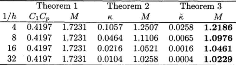
Table 1 and 2 show verification results. The bold letters indicate the smallest $M$ in the theorems.

Table 1: Verification results for $b=\sin(\pi x)$, $c=1,$ $\rho=1.0035(1/h=32)$

Theorem1 Theorem 2 Theorem 3

$\frac{1/hC_{1}C_{p}M\kappa M\tilde{\kappa}M}{40.41971.72310.10571.25070.02581.2186}$

8 0.4197 1.7231 0.0464 1.1106 0.0065 1.0976

16 0.4197 1.7231 0.0216 1.0521 0.0016 1.0461

32 0.4197 1.7231 0.0104 1.0258 0.0004 1.0229

Table 2: Verification results for $b=-\sin(\pi x)$, $c=-5,$ $\rho=2.0001(1/h=32)$

Theorem1 Theorem2 Theorem3

$\frac{1/hC_{1}C_{p}M\kappa M\tilde{\kappa}M}{40.82505.71160.22482.51550.15392.4918}$

8 0.8250 5.7116 0.0770 2.1125 0.0393 2.1122

16 0.8250 5.7116 0.0293 2.0280 0.0099 2.0285

32 0.8250 5.7116 0.0123 2.$00S2$ _0.0025

_2.0084

3.4.2 Two-dimensionalnon-self adjoint operators

Consider the case for

$b=R[_{x-1/2}^{-y+1/2}], c\in \mathbb{C}, \Omega=(0,1)\cross(0,1)$ ₍₂₂₎

We take linear anduniformtriangularmesheson$\Omega$with the element sidelength

$h>0$foragivenfinite

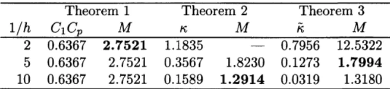
element mesh. We can take $C(h)=0.493h$ and $C_{p}=1/(\pi\sqrt{2})$. _{Table 3, 4, and 5 show verification}

Table3: Verification results for$R=4,$ $c=0,$ $\rho=1.0001(1/h=10)$

Theorem1 Theorem 2 Theorem 3

$\frac{1/hC_{1}C_{p}M\kappa M\tilde{\kappa}M}{20.63672.75211.1835-0.795612.5322}$

5 0.6367 2.7521 0.3567 1.8230 0.1273 1.7994

10 0.6367 2.7521 0.1589 1.2914 0.0319 1.3180

Table4: Verification results for$R=6.75,$ _$c=-1-1.5i,$ $\rho=1.0487(1/h=10)$

Theorem1 Theorem 2Theorem3

$\frac{1/hC_{1}C_{r}M\kappa M\tilde{\kappa}M}{41.1658-1.0408-0.892823.7783}$

5 1.1658 – 0.7608 5.6411 0.5721 5.1856

10 1.1658 – 0.3081 1.7124 0.1433 1.8585

3.5

Report for

estimation

(2)

Weconsider three computer-assisted procedures to verifythe invertibilityof second orderlinear elliptic operatorswithabound for thenormofits inverse. Although it has thelimitation,the method of Theorem 1 does not needthe computationof$\rho$ (2-norm). Themethod based on Theorem3 has the second order

for$C(h)$ _when$b\in W^{1,\infty}(\Omega)$ and some verificationresults show that it could beanalternativeofTheorem

2, especially,some confirmation of the only invertibility for$\mathscr{L}$arequite essential. We stillconcludeour

second approach of Theorem 2 is robust and reliable than other two approaches.

4

Estimation

(3)

Nowwe consideran upper bound$M$ safisfying

$\Vert u\Vert_{H_{0}^{1}(\Omega)}\leq M\Vert \mathscr{L}u\Vert_{L^{2}(\Omega)} \forall u\in H(\triangle;L^{2}(\Omega))$

.

Wehave three approaches.

4.1

1st

estimation

of (3)

Our firstresult is adirect applicationof Theorem 2.

Theorem 4. [13, Theorem 2.3] If$\kappa=C(h)(\rho C_{1}K+C_{2})<1$ _then $\mathscr{L}$is invertible and $M>0$of

(3) is obtained by

$M= \frac{C_{p}}{1-\kappa}\Vert[^{\rho(1-C_{2}C(h))}\rho C_{1}C(h) \rho_{1}K]\Vert_{2}$

In Theorem 4, it is expected that $M arrow C_{p}\max\{\rho$, 1$\}.$

4.2

2nd

estimation

of

(3)

For

$\hat{\rho}:=\Vert D^{H/2}G^{-1}L^{1/2}\Vert_{2}$, (23)

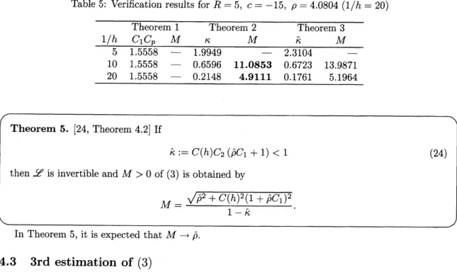
Table5: Verification resultsfor $R=5,$ $c=-15,$ $\rho=4.0804(1/h=20)$

Theorem 1 Theorem 2 Theorem 3

$\frac{1/hC_{1}C_{p}M\kappa M\tilde{\kappa}M}{51.5558-1.9949-2.3104-}$ 10 1.5558 – 0.6596 11.0853 0.6723 13.9871 20 1.5558 – 0.2148 4.9111 0.1761 5.1964 Theorem 5. [24, Theorem4.2] If $\hat{\kappa}$ :$=C$ (ん)$C$₂$(\hat{\rho}C_{1}+1)<1$ ₍₂₄₎ then $\mathscr{L}$is

invertible and $M>0$ of(3) is obtained by

$M= \frac{\sqrt{\hat{\rho}^{2}+C(h)^{2}(1+\hat{\rho}C_{1})^{2}}}{1-\hat{\kappa}}.$

InTheorem5, it isexpectedthat $Marrow\hat{\rho}.$

4.3

3rd

estimation

of

(3)

We alsopresent the following estimate basedon afixed-point formulation.

Theorem 6. [4, Theorem 3] If$\kappa=C(h)(\rho C_{1}K+C_{2})<1$ _then$\mathscr{L}$is invertible and

$M>0$of (3)

is obtained by

$M= \frac{\sqrt{\mathscr{J}(C_{p}+C(h)(K-C_{p}C_{2}))^{2}+C(h)^{2}(1+\rho C_{p}C_{1})^{2}}}{1-\kappa}.$

InTheorem 6, itisexpectedthat $Marrow C_{p}\rho.$

Comparing three theorems for (3), Theorem 5 couldconverge to the exact operatornorm for$\mathscr{L}^{-1}.$

Because of it holds that $\hat{\rho}\leq C_{p}\rho$, when$\hat{\rho}\sim C_{p}\rho$, Theorem 6 would apply suffient “good” _$M$ with low computationalcost. $Rom$_{the actualcomputational pointofview, sincethe criterion}$\hat{\kappa}<1$is sometimes harder than $\kappa<1$ forfixed $h$ experimentally, Theorem4 _and6 _have

aroomto be effective.

4.4

Numerical

examples

Our numerical environment and $S_{h}$ for

one-

or two-dimensional operators are same as the _previous

section.

4.4.1 One-dimensional operators

Table 6, 7, 8, and9 showverificationresults forsome $b(x)=r\sin(\pi x)$ and $c\in \mathbb{R}$ in

$\Omega=(0,1)$.

4.4.2 Two-dimensional non-self-adjoint operators

Consider thecasefor (22). Table 10 and 11 showverification results.

4.4.3 Two-dimensional operators

We nowreport on a case for $b=$ _{O. Consider an operator:} $\mathscr{L}=-\triangle-1-2u_{h}+3au_{h}^{2}$ which is the

linearizedthe equation

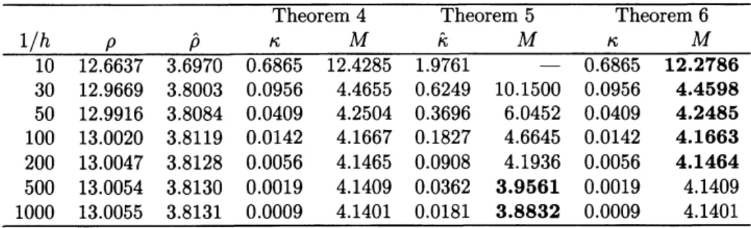
Table 6: Verificationresults for $b=2.5\sin(\pi x)$, $c=-10$

Theorem4 Theorem 5Theorem6

$\frac{1/h\rho\hat{\rho}\kappa M\hat{\kappa}M\kappa M}{1012.66373.69700.686512.42851.9761-0.686512.2786}$ 30 12.9669 3.8003 0.0956 4.4655 0.6249 10.1500 0.0956 4.4598 50 12.9916 3.8084 0.0409 4.2504 0.3696 6.0452 0.0409 4.2485 100 13.0020 3.8119 0.0142 4.1667 0.1827 4.6645 0.0142 4.1663 200 13.0047 3.8128 0.0056 4.1465

0.0908

4.1936 0.0056 4.1464 500 13.0054 3.8130

0.0019

4.1409

0.0362

3.9561

0.0019

4.1409 1000 13.0055 3.8131 0.0009 4.1401 0.0181 3.8832 0.0009 4.1401

Table 7: Verification results for$b=-20\sin(\pi x)$, $c=-20.$

Theorem4 Theorem 5Theorem 6

$\frac{1/h\rho\hat{\rho}\kappa M\hat{\kappa}M\kappa M}{102.64200.35523.9293-6.8074-3.9293-}$ 30 2.5044 0.3542 0.5592 1.8684 2.2167 – 0.5592 1.5439 50 2.4950 0.3542 0.2518 1.0293 1.3246 – 0.2518 0.9502 100 2.4911 0.3542 0.0948 0.8417 0.6603 1.0469 0.0948 0.8249 200 2.4911 0.3542 0.0396 0.8040 0.3296 0.5289 0.0396 0.8002 500 2.4899 0.3542 0.0140 0.7943 0.1318 0.4080 0.0140 0.7938 1000 2.4899 0.3542 0.0067 0.7930 0.0659 0.3792 0.0067 0.7929

at two finite element approximate solutions$u_{h}$ whosenamed “lower” and (upper.”

Table 12and 13 showverification results.

4.5

Report

for

estimation

(3)

Thecomputer-assisted procedure (Theorem 6) isourlatestapproachtocomputeaverified bound of the normfor secondorder linear elliptic operators$\mathscr{L}$. The criterionfor theinvertibilityof$\mathscr{L}$isthesame as

Theorem 4, however,it hasno limitation such that the lower bound of$M$ is not less than 1. Although

the proposed procedure would notconvergetoits exact operator norm,someverification examples show

that it has abetter bound than the approach in Theorem 5. We conclude that our proposed method

should be

a

bridge the gap between the two previous approaches, and

one

may choicean appropriate

proceduretaking into consideration given problem orcomputational cost, and

so

on.

5

Estimation

(4)

Finally weconsideran upper bound $M$safisfying

$\Vert\triangle u\Vert_{L^{2}(\Omega)}\leq M\Vert \mathscr{L}u\Vert_{L^{2}(\Omega)}, \forall u\in H(\triangle;L^{2}(\Omega))$.

Wehavetwo approaches.

5.1

1st estimation

of (4)

Table8: Verificationresultsfor $b=\sin(\pi x)$, $c=100.$

Theorem4 Theorem 5Theorem6

$\frac{1/h\rho\hat{\rho}\kappa M\hat{\kappa}M\kappa M}{100.91830.05001.1665-0.35160.15081.1665-}$ 30 0.9911 0.0499 0.1458 0.4977 0.0577 0.0608 0.1458

0.3920

50 0.9969 0.0499 0.0553 0.4060 0.0275 0.0542 0.0553 0.3426 100 0.9992 0.0499 0.0155 0.3568 0.0111 0.0512 0.0155 0.3242 200 0.9998 0.0499 0.0047 0.3365 0.0049 0.0504 0.0047 0.3198 500 1.0000

0.0499

0.0012 0.3254 0.0018 0.0501 0.0012 0.3186 1000 1.0000 0.0499 0.0005 0.3218 0.0009 0.0500 0.0005 0.3184

Table9: Verificationresults for $b=\sin(\pi x)$, $c=-10.$

Theorem4 Theorem5Theorem 6

$\frac{1/h\rho\hat{\rho}\kappa M\hat{\kappa}M\kappa M}{1094.962129.62612.1281-5.2424-2.1281-}$ 30

231.4257

72.4346 0.5767 172.3900 3.5678 – 0.5767 172.4427 50 261.5470 81.8835 0.2366 108.4156 2.3262 – 0.2366 108.4277 100 276.7469 86.6517 0.0641 93.8348 1.1938 – 0.0641 93.8375 200 280.8268 87.9316 0.0171 90.7977 0.5964 217.8445 0.0171 90.7983 500 281.9909 88.2967 0.0032 89.9844 0.2373 115.7653 0.0032 89.9846 1000 282.1580 88.3491 0.0010 89.8696 0.1184 100.2071 0.0010 89.8697

Theorem 7. If$\kappa_{7}$ $:=C(h)C_{2}(\rho_{10}C_{1}+1)<1$ then

$\mathscr{L}$isinvertible and$M>0$of(4) isobtained by

$M=1+\Vert b\Vert_{L^{\infty}(\Omega)^{d}}A_{1}+\Vert c\Vert_{L^{\infty}(\Omega)}A_{0},$

where

$A_{0}= \frac{\rho_{00}+C(h)^{2}(1+\rho_{10}C_{1})}{1-\kappa_{7}}, A_{1}=\frac{\sqrt{p_{10}^{2}+C(h)^{2}(1+\rho_{10}C_{1})^{2}}}{1-\kappa_{7}}.$

5.2

2nd

estimation

of (4)

Note that if$E$_{is positive definite, by using}$E=E^{1/2}E^{H/2}$_{, it is true that}

Table 10: Verification results for$R=10,$ $c=-10-5i.$

$\overline{Theorem4}$

Theorem5Theorem6 $\frac{1/h\rho\hat{\rho}\kappa M\hat{\kappa}M\kappa M}{51.70390.36562.3287-3.6305-2.3287-}$ 10 1.7751 0.3946 0.7724 1.8734 1.7974 –

0.7724

1.6510 20

1.7941

0.4025

0.2814

0.5384

0.8798

3.4926

0.2814

0.5033 50 1.7995 0.4047 0.0869 0.4222 0.3456 0.6227 0.0869 0.4174 100 1.8001

0.4050

0.0392 0.4092 0.1716

0.4897

0.0392

0.4082 130 1.8004 0.4051 0.0294 0.4076 0.1318

0.4670

0.0294 0.4070

Table 11: Verification results for $R=10,$ $c=15.$

$\overline{Theorem4}$

Theorem5Theorem6 $\frac{1/h\rho\hat{\rho}\kappa M\hat{\kappa}M\kappa M}{50.97320.12701.8758-1.9610-1.8758-}$ 8 0.9903 0.1276 0.9032 3.3368 1.1493 – 0.9032 2.6387 10 0.9939 0.1277 0.6488 0.8671 0.8987 1.6951 0.6488 0.6589 20 0.9986

0.1279

0.2497 0.3543

0.4284

0.2453

0.2497

0.2760 50

0.9999

0.1279 0.0818 0.2632

0.1663

0.1559

0.0818

0.2316 100 1.0001 0.1279 0.0379 0.2426 0.0823 0.1400

0.0379

0.2267

5.3

Numerical

examples

Considerthe casefor two-dimensionalnon-self-adjoint operators (22). Our numericalenvironment and

$S_{h}$ issame

as

the previoussection. Table 14 and 15 showverification results.

5.4

Report

for

estimation

(4)

Weproposetwocomputer-assistedprocedures to computea verifiedbound $M>0$satisfying (4). Some

verification examples show that Theorem 8 hasabetter bound than the approach in Theorem7. Ifwe

are indifferent to computationalcosts, instead ofan estimation

$\Vert b\cdot\nabla uh+cu_{h}\Vert_{L^{2}(\Omega)}\leq M_{h}(C(h)C_{2}\Vert\triangle u\Vert_{L^{2}(\Omega)}+\Vert f\Vert_{L^{2}(\Omega)})$

in the proofofthe Theorem 8, it canbe possible touse a bound such that

$\Vert b\cdot\nabla u_{h}+cu_{h}+f\Vert_{L^{2}(\Omega)}\leq\hat{M}_{h}\Vert f\Vert_{L^{2}(\Omega)}$

with numerically determined $\hat{M}_{h}>0$directly (more constructive).

Acknowledgments

This work was supported by a Grant-in-Aid from the Ministry ofEducation, Culture, Sports, Science

and Technology of Japan (No. 24340018,23740074, and 24540151).

References

[1] P.G. Ciarlet, The Finite Element Method

_for

Elliptic Problems, North-Holland, Amsterdam, 1978.

[2] K. Hashimoto, K. Nagatou, and M.T. Nakao, A computational approach to constructive a priori

error

estimate for finite element approximationsofbi-harmonic problems in

nonconvex

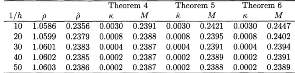
polygonal

Table 12: Verification results for “lower” $u_{h}$ at $a=0.001.\hat{\rho}/(C_{p}\rho)\sim 0.9995(1/h=50)$.

Theorem4 Theorem 5Theorem 6

$\frac{1/h\rho\hat{\rho}\kappa M\hat{\kappa}M\kappa M}{101.05860.23560.00300.23910.00300.24210.00300.2447}$

20 1.0599 0.2379 0.0008

0.2388

0.0008

0.2395

0.0008 0.2402

30 1.0601 0.2383 0.0004 0.2387 0.0004 0.2391 0.0004 0.2394

40 1.0602 0.2385 0.0002 0.2387 0.0002 0.2389 0.0002 0.2391

50 1.0603 0.2386 0.0002 0.2387 0.0002 0.2388 0.0002 0.2389

Table 13: Verification results for “upper” $u_{h}$ at$a=0.001.\hat{\rho}/(C_{p}\rho)\sim 0.6040(1/h=50)$

.

Theorem4 Theorem 5Theorem6

$\frac{1/h\rho\hat{\rho}\kappa M\hat{\kappa}M\kappa M}{102.59480.35451.1823-0.77221.96681.1823-}$

20 2.6622 0.3624 0.2856 0.9204 0.1861 0.4756 0.2856 0.8883

30 2.6758 0.3640 0.1262 0.7216 0.0822 0.4087 0.1262 0.7074

40 2.6807 0.3645 0.0709 0.6671 0.0461 0.3887 0.0709 0.6590

50 2.6830

0.3648

0.0453

0.6438

0.0295

0.3800 0.0453

0.6386

[3] F.Kikuchi and X. Liu, Determination ofthe Babuska-Aziz constant for the linear triangularfinite

element, Japan Journal

_of

Industrial and Appl\’ied Mathematics 2375-82 (2006).

[4] T. Kinoshita, Y. Watanabe, and M.T. Nakao, Some remarks onthe rigorousestimation of inverse

linear elliptic operators,submitted.

[5] K. Kobayashi, A constructivea priori error estimation for finite element discretizations in a

non-convex domain using singular functions, Japan Journal

_of

industrial and Applied Mathematics 26

493-516 (2009).

[6] X. Liu and S. Oishi, Verified eigenvalue evaluation for the Laplacian over polygonal domains of

arbitrary shape, SIAMJournal on Numerical Analysis 511634-1654 (2013).

[7] M.T. Nakao,Computable$L^{\infty}$ errorestimates inthe finite element method withapplicationto

non-linear elliptic problems, in ContributionsinNumericalMathematics,pp. 309-319,ed.R. P. Agarwal,

World Scientific, Singapore, 1993.

[8] M.T. Nakao and N. Yamamoto, Numerical verificationof solutions for nonlinear elliptic problems using$L^{\infty}$ residual method,Journal

of

Mathematical Analysis and Applications217246-262(1998). [9] M.T. Nakao, N. Yamamoto, and S. Kimura, On best constant in the error bound for the $H_{0^{-}}^{1}$

projection intopiecewise polynomialspaces, Journal

_of

Approximation Theory93491-500 (1998).

[10] M.T.Nakaoand N. Yamamoto,Aguaranteed boundofthe optimalconstantintheerrorestimates

forlineartriangular element,in Topics inNumericalAnalysis With Special Emphasis on Nonlinear

Problems, eds. G. Alfeld, and X. Chen, pp. 163-173, Computing Supplement, vol. 15, Springer,

Wien, NewYork,2001.

[11] M.T. Nakaoand N. Yamamoto, Aguaranteed bound of the optimalconstant intheerrorestimates

for linear triangular element Part II: Details, inPerspectives onEnclosure Methods, eds.U.Kulisch,

R. Lohner, and A. Facius, pp. 265-276, Springer, Wien, NewYork, 2001.

[12] M.T. Nakao, Numerical verification methods for solutions of ordinary and partialdifferential

Table 14: Verification resultsfor $R=20,$ $c=0.$ $\overline{\frac{1/hTheorem7Theorem8M_{h}\rho_{10}\rho_{00}A_{0}A_{1}}{20-3.53860.58430.22380.0501--}}$ 30 108.0393 2.5102 0.5854 0.2242 0.0503 1.6592 7.5689 40 12.9217 2.1922 0.5861 0.2243 0.0504 0.1867 0.8430 50 8.7114 2.0372 0.5865 0.2244 0.0504 0.1214

0.5453

100

5.4943

1.7847 0.5872 0.2244 0.0504

0.0712

0.3178

130 5.0987 1.7350 0.5873 0.2244

0.0504

0.0650 0.2899

Table 15: Verificationresults for$R=10,$ _$c=-10-10i.$

$\overline{\frac{1/hTheorem7Theorem8M_{h}\rho_{10}\rho_{00}A_{0}A_{1}}{2016.30723.26711.04510.31720.07120.33141.5020}}$ 30 7.7991 2.7135 1.0469 0.3177 0.0714 0.1483 0.6651 40 6.3207 2.5057 1.0475 0.3179 0.0715 0.1164 0.5199 50 5.7107 2.3968 1.0478 0.3180 0.0715 0.1032 0.4600 100 4.8430 2.2077 1.0482 0.3181 0.0716 0.0843 0.3750 130 4.6888 2.1683 1.0483 0.3181 0.0716 0.0809 0.3599

[13] M.T. Nakao, K. Hashimoto, and Y. Watanabe, A numerical method to verify the invertibility of

linearelliptic operatorswith applications tononlinearproblems, Computing 751-14 (2005).

[14] M.T. Nakao, K. Hashimoto, and K. Kobayashi, Verified numerical computation of solutions for the stationary Navier-Stokes equation in nonconvex polygonal domains, Hokkaido Mathematical

Journal

_36777-799.

(2007).

[15] M.T. Nakao, K. Hashimoto, and K. Nagatou, A computational approachto constructive a priori

and a posteriori error estimates for finite element approximations of bi-harmonic problems, in

Proceedings

_of

the

_4th

JSIAM-SIMAI Seminar on Industrial and Applied Mathematics, GAKUTO

International Series, Mathematical Sciences and Applications, vol. 28, pp. 139-148, Gakkotosho,

Tokyo, Japan, 2008.

[16] M.T. Nakao and Y. Watanabe, Numerical verification methods for solutions of semilinear elliptic

boundary valueproblems, Nonlinear Theory and Its Applications, IEICE 22-31 (2011).

[17] M.T. Nakao, Y. Watanabe, T. Kinoshita, T. Kimura, and N. Yamamoto, Some considerations of the invertibility verifications for linear elliptic operators, Japan Journal

_of

Industral and Applied

Mathematics, toappear.

[18] M. Plum, Explicit$H_{2}$-estimatesand pointwiseboundsforsolutions of second-orderellipticboundary

valueproblems, Journal

of

MathematicalAnalysis and Applications 16536-61 (1992).

[19] M.Plum,Numericalexistenceproofsandexplicitbounds for solutions of nonlinearellipticboundary value problems, Computing 4925-44 (1992).

[20] M. Plum, Existence and multiplicity proofs for semilinear elliptic boundary value problems by computer assistance, Jahresbericht derDeutschen Mathematiker Vereinigung 11019-54 (2008).

[21] S.M. Rump, INTLAB – INTerval LABoratory, in Developments in Reliable Computing, ed.

T. Csendes, pp. 77-104, Kluwer AcademicPublishers, Dordrecht, 1999.

http:$//www$_{.ti3. tu-harburg.}$de/rump/$

[22] S.M. Rump,Verified bounds for singularvalues, inparticularfor the spectralnormofamatrix and itsinverse, BIT Numerical Mathematics 51367-384(2011).

[23] Y. Watanabe, N. Yamamoto, M.T. Nakao, and T. Nishida, A numerical verification ofnontrivial solutions fortheheatconvectionproblem, Journal

_of

Mathematical Fluid Mechanics61-20 (2004).

[24] Y. Watanabe,T. Kinoshita,and M.T. Nakao, Aposterioriestimates ofinverseoperatorsfor

bound-ary value problems in linear elliptic partial differential equations, Mathematics

_of

Computation 82

1543-1557(2013).

[25] Y. Watanabe, K. Nagatou, M. Plum, and M.T. Nakao, Verified computations ofeigenvalue

exclo-suresforeigenvalue problems in Hilbert spaces, SIAMJournal on Numerical Analysis 52975-992

(2014).

[26] N. Yamamoto and M.T. Nakao, Numerical verifications of solutions for elliptic equations in

non-convexpolygonal domains, Numerische Mathematik65503-521 (1993).

[27] N. Yamamoto and K. Hayakawa, Error estimation with guaranteed accuracy of finite element

method in

nonconvex

polygonal domains, Journal

_of

Computationaland Applied Mathematics 159

173-183 (2003).

[28] N. Yamamoto and K. Gemma, On errorestimation of finite element approximations to theelliptic

equations in nonconvex polygonal domains, Journal

_of

Computational and Applied Mathematics