On the plasticity models with some threshold functions (Theory of Evolution Equation and Mathematical Analysis of Nonlinear Phenomena)
10
0
0
全文
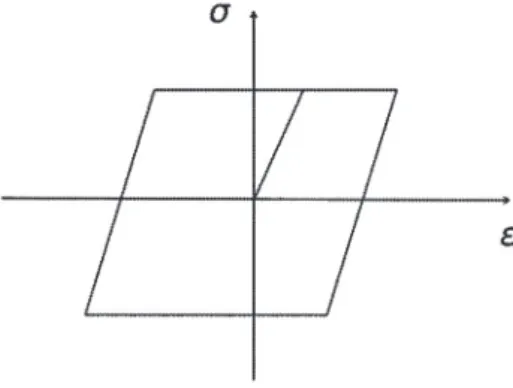
(2) 61 61. Figure 1: The relation of stress and strain. We define the yield function. F. that determines whether the stress is yielding situation,. by. F(\sigma)<g F(\sigma)=g where,. g. \Rightarrow \Rightarrow. only elastic, yielding situation,. (2.ı) (2.2). is a non‐negative function that is called the threshold function. For example,. F( \sigma)=\frac{1}{2}|\tau^{D}|^{2} \tau_{ij}^{D} := \tau_{ij}-(1/3)\sum_{k=1}^{3}\tau_{kk}\delta_{ij} for i,j=1,2,3 \tau\in \mathb {R}_{sym}^{3\cros 3} , the symbol \delta_{ij} is the Kronecker delta.. where,. and |\tau|^{2}. := \sum_{i,j=1}^{3}\tau_{ij}\tau_{ij}. for all. We call the perfect plasticity model, if The threshold function is independent in. \varepsilon. (Figure 2). In this case, the relation \{(2.1),(2.2)\} is presented by the following formulation;. .;. Figure 2: The relation of stress and strain for the perfect plasticity.
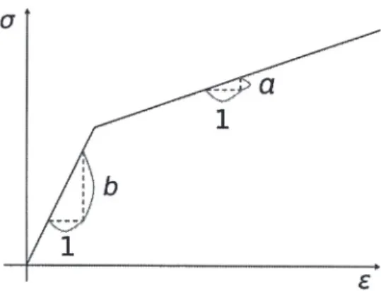
(3) 62. \{begin{ar y}{l F(\sigma)<g \Rightarow\frac{prtial\vrepsilon_{p}\artil}=0, F(\sigma)=gnd\frac{prtial\sgma}{\prtial}=0 \Rightarow\frac{prtial\vrepsilon_{p}\artil}\geq0. \end{ar y}. Namely, we get the following the Moreau sweeping process form. \frac{\partial\varepsilon_{p}{\partialt}\in\partialI_{Z}(\sigma) , where,. Z. is a time‐dependent closed convex set defined by. (2.3) Z. :=\{\tau\in \mathbb{R}_{sym}^{3\cross 3} : (1/2)|\tau^{D}|^{2}\leq. g\} . Moreover, I_{Z} is the indicator function of Z, \partial I_{Z} is the subdifferential of I_{Z}.. Moreover, we consider the two conditions for the strain. The first condition is the ad‐. ditive decomposition of strains, namely, the strain can be expressed by the decomposition of elastic and plastic parts;. \varepsilon(u)=\varepsilon_{e}+\varepsilon_{p} .. (2.4). The second condition is that the elastic strain is linear with respect to stress; \varepsilon_{e}=L\sigma ,. where,. L. is the. 3\cross 3. (2.5). matrix. Hence, we combine three conditions (2.3), (2.4) and (2.5),. after that we can get the equation of \sigma . Indeed, taking the time derivative of first equation using the second equation, and then the third equation becomes the following inclusion;. L\frac{\partial\sigma}{\partialt}+\partialI_{Z}(\sigma)\ni\varepsilon(\frac{ \partialu}{\partialt}) . 2.2. (2.6). Hardening. Next, we recall the hardening problem in one dimensional space, which is derived by. Visintin [5]. His idea is the characteristic of yielding situation. We put. a. and. b. are slopes. of strain for stress, respectively with 0\leq a<b . When the strain consists of only the elastic strain that is on the elastic region, the slope is equal to b . When the strain consists of the elastic strain and the plastic strain that is on the plastic region, the slope is equal. to. a. (Figure 3). In this case, the threshold value is equal to g+a\varepsilon . Therefore, we can get. the following new expression of the plastic strain. \frac{\partial\varepsilon_{p}{\partialt}\in\partialI_{Z}(\sigma- a\varepsilon) ,. (2.7). indeed, these conditions are equivalent, \sigma-a\varepsilon\in Z \Leftrightarrow \sigma\in Z+a\varepsilon.. Hence, we combine three conditions (2.7), (2.4) and (2.5), we get the new equation of \sigma ;. \frac{\partial\sigma}{\partialt}+\partialI_{Z}(\sigma- \varepsilon(u) \ni b\varepsilon(\frac{\partialu}{\partialt}) . As the remark, in 1D case, on the previous perfect plasticity model (3.2), we take and b=1/L.. (2.8) a=0.
(4) 63. Figure 3: The relation of stress and strain in hardening process. 3. The Known result of the perfect plasticity case. In this section, we introduce the existence theorem for the perfect plasticity problems of some type. For each theorem, we used by the method of variational inequality. The constraint is described by the Moreau sweeping process form which is well‐known in the. abstract evolution equations (c.f.[4]).. 3.1. The classical problem by Duvaut‐Lions. In this section, we recall the problem of perfect plasticity is derived by Duvaut and. Lions [1]. The domain. \Omega. is the bounded set in. \mathb {R}^{3}. with the smooth boundary. \Gamma=\partial\Omega. which consists of \Gamma=\Gamma_{D}\cup\Gamma_{N} , and \Gamma_{D}\cap\Gamma_{N}=\emptyset with |\Gamma_{D}|>0 and |\Gamma_{N}|>0. \nu denotes the unit normal vector outward from \Gamma . The unknown functions u=(u_{1}, u_{2}, u_{3}) , \sigma=\{\sigma_{ij}\}_{i,j=1,2,3} , describe the displacement and the stress tensor, respectively. The strain \varepsilon(u)=\{\varepsilon_{i,j}\}_{i,j=1,2,3} depending by displacement u , is defined by. \varepsilon_{i,j}=\frac{1}{2}(\frac{\partialu_{i}{\partialx_{j}+ \frac{\partialu_{j}{\partialx_{i}) for. ,. i,j=1,2,3.. We consider the model of perfect plasticity. To find. v. :=\partial u/\partial t and. \frac{\partial v}{\partial t}=div\sigma+f in Q:=(0,T)\cross\Omega , \frac{\partial\sigma}{\partial t}+\partial I_{Z}(\sigma+\sigma_{*}) \ni\varepsilon(v)+h in Q ,. \sigma. satisfying. (3.9) (3.10). where f : Qarrow \mathbb{R}^{3}, h : Qarrow \mathbb{R}_{sym}^{3\cros 3} , and \sigma_{*} : Qarrow \mathbb{R}_{sym}^{3\cros 3} are given functions in Q, \mathb {R}_{sym}^{3\cros 3} stands for the 3\cross 3 symmetric matrix. With the help of h and \sigma_{*} , we can translate the problem to the homogeneous boundary value problem. The operator div is defined by div\tau :=(div\tau_{1}., div\tau_{2}., div\tau_{3}.) for all \tau\in \mathbb{R}_{sym}^{3\cros 3} , where div\tau_{i}. := \sum_{j=1}^{3}\partial\tau_{ij}/\partial x_{j} for i=1,2,3 . The first equation (3.9) is derived by the conservation law of momentum. The.
(5) 64 second equation (3.10) ensures the property of perfect plasticity, where we assume the additive decomposition of strain as Section 2.1.. We use the following notation: H :=L^{2}(\Omega)^{3}, V := { z\in H^{1}(\Omega)^{3}:z=0 a.e. on \Gamma_{D} }, with their inner products (\cdot, \cdot)_{H}, (\cdot, \cdot)_{V} , and the norm |\cdot|_{H} , where |\cdot|_{V} is defined by. |z|_{V}. :=\{ sum_{i,j=1}^{3}\int_{\Omega}|\frac{\partialz_{i} \partialx_{j}|^{2}dx \}^{\frac{1}2}. for all z\in V.. Denote the dual space of V by V^{*} with the duality pair \{\cdot, \cdot\rangle_{V^{*},V} . Moreover, we define the following bilinear form: ( \cdot, \cdot) : V\cross Varrow \mathbb{R}. (z,\tilde{z}):=\sum_{i,j=1}^{3}\int_{\Omega}\frac{\partialz_{i} \partial x_{j}\frac{\partial\tilde{z}_{i}\partialx_{j}dx We also define 0. for all. \mathbb{H}:=\{\tau :=\{\tau_{ij}\} : \tau_{ij}\in L^{2}(\Omega), \tau_{ij}= \tau_{ji}\},. z,\tilde{z}\in V.. :=\{\tau\in \mathbb{H}. V. :. div\tau\in H,. \tau_{i}.\cdot v=. a.e. on \Gamma_{N}\} with their inner products. (\tau,\tilde{\tau})_{\mathb {H} (\tau,\tilde{\tau})_{V}. :=\sum_{i,j=1}^{3}\int_{\Omega}\tau_{ij}\tilde{\tau}_{ij}dx :=(\tau,\tilde{\tau})_{\mathb {H}+(div\tau,div\tilde{\tau})_{H}=(\tau,\tilde {\tau})_{\mathb {H}+\sum_{i,j=1}^{3}\int_{\Omega}\frac{\partial\tau_{ij} {\partialx_{j}\frac{\partial\tilde{\tau}_{ij}{\partialx_{j}dx for all. \tau,\tilde{\tau}\in \mathbb{H},. for all. \tau,\tilde{\tau}\in V.. The following convex constraint plays an important role in this paper. For each t\in[0, T],. \tilde{K}(t). :=. {. \tau\in \mathbb{H}. : \frac{1}{2}|\tau^{D}(x)|^{2}\leq g(t, x) for. a.a.. x\in\Omega. },. Finally, we recall an important relation. For each z\in V,. K(t) :=\tilde{K}(t)-\sigma_{*}(t) \tau\in V ,. .. the following relation. holds:. (\varepsilon(z), \tau)_{\mathbb{H}}+(div\tau, z)_{H}=0 .. (3.11). This is called the Gauss‐Green relation.. In the paper [1], the threshold function. g. is a constant function. Duvaut and Lions. showed the existence of solutions for the perfect plasticity model.. Proposition 3.1.. We assume that the following conditions hold;. f\in W^{1,2}(0, T;H) h\in W^{1,2}(0, T;\mathbb{H}) and. \sigma_{*}. ,. ,. is independent of time t . Then there exists an unique pair of functions (v, \sigma) such. that. v, v'\in L^{\infty}(0, T;H). \sigma, \sigma'\in L^{\infty}(0, T;\mathbb{H}). ,. ,.
(6) 65 v_{i}\in L^{\infty}(0, T;L^{2}(\Omega)). ,. \sigma_{i,j}\in L^{\infty}(0, T;L^{2}(\Omega)). ,. and that satisfy. (v'(t), z)_{H}-(div(a(t)), z)_{H}=(f(t), z)_{H}. for all z\in V,. and. (\sigma'(t), \sigma(t)-\tau)_{\mathbb{H}}-(\varepsilon(v(t)), \sigma(t)-\tau)_{ \mathbb{H}}\leq(h(t), \sigma(t)-\tau)_{\mathbb{H}} for a.a.. 3.2. t\in(0, T). with. v(0)=v_{0}. in H and. \sigma(0)=\sigma_{0}. for all \tau\in V. in \mathbb{H}.. The perfect plasticity problem with the threshold depending on time. We consider the case of the threshold function g=g(t) depending on time, because, the threshold function depend on the unknown function in the target hardening problem. We use the same notation in the above section.. Definition 3.1. For each \kappa\in(0,1 ] and \nu\in(0,1 ], the pair (v, \sigma) is called a solution of modified problem for (3.9) and (3.10) in the sense of variational inequality if. v\in H^{1}(0, T;H)\cap L^{\infty}(0, T;V)\cap L^{2}(0, T;H^{2}(\Omega)^{3}). \sigma\in H^{1}(0, T;\mathbb{H})\cap L^{2}(0, T;V) ,. \sigma(t)\in K(t). ,. for all t\in[0, T],. and they satisfy. (v'(t), z)_{H}+\nu((v(t), z))-(div(a(t)), z)_{H}=(f(t), z)_{H} for all z\in V, (\sigma'(t), \sigma(t)-\tau)_{\mathbb{H}}+\kappa(\sigma(t), \sigma(t)-\tau)_{V} -(\varepsilon(v(t)), \sigma(t)-\tau)_{\mathbb{H}} \leq(h(t), \sigma(t)-\tau)_{\mathbb{H}} for all \tau\in K(t)\cap V for. a.a.. t\in(0, T) with v(0)=v_{0} in. Proposition 3.2.. H. and \sigma(0)=\sigma_{0} in. \mathbb{H}.. We assume that (A1)-(A5) hold;. (A1) f\in L^{2}(0, T;H) and h\in L^{2}(0,T;\mathbb{H}) ;. (A2) v_{0}\in V and \sigma_{0}\in K(0)\cap V ; (A3) \sigma_{*}\in H^{1}(0,T;V) ; (A4) g\in H^{1}(0, T;C(\overline{\Omega}))\cap C(\overline{Q}) ;. (A5) There exist two constants C_{1}, C_{2}>0 such that 0<C_{1}\leq g(t, x)\leq C_{2}. for all. (t, x)\in\overline{Q}..
(7) 66 Then, there exists a unique solution (v, \sigma) of modified problem for (3.9) and (3.10) in the sense of variational inequality.. Let us remove the parameter \kappa\in(0,1 ]. In this case, the problem is the same as the Moreau sweeping process.. Definition 3.2. For each \nu\in(0,1 ], the pair (v, \sigma) is called a solution of the viscous perfect plasticity model for (3.9) and (3.10) if. v\in H^{1}(0, T;V^{*})\cap L^{\infty}(0, T;H)\cap L^{2}(0, T;V). \sigma\in H^{1}(0, T;\mathbb{H}) ,. \sigma(t)\in K(t). ,. for all t\in[0, T],. and they satisfy. \langle v'(t), z\rangle_{V^{*},V}+\nu((v(t), z))+(\sigma(t), \varepsilon(z))_{\mathbb{H}}= (f(t), z)_{H}. (\sigma'(t), \sigma(t)-\tau)_{\mathbb{H}}-(\varepsilon(v(t)), \sigma(t)-\tau)_{ \mathbb{H}}\leq(h(t), \sigma(t)-\tau)_{\mathbb{H}} for. a.a.. t\in(0, T) with v(0)=v_{0} in. H. and \sigma(0)=\sigma_{0} in. for all z\in V,. for all \tau\in K(t). \mathbb{H}.. We replace (A3) by (A3’): (A3 ) \sigma_{*}\in H^{1}(0, T;\mathbb{H}) .. Proposition 3.3. Under assumptions (A1), (A2), (A3 ), (A4), and (A5), there exists a unique solution (v, \sigma) of the viscous perfect plasticity model for (3.9) and (3.10). The proposition 3.2 and 3.3 is showed by Fukao and Kano in [2].. 3.3. The perfect plasticity weakly problem with the threshold depending on time. To relax assumption (A4) on. g. with respect to time regularity, we recall the concept of. the weak variational formulation:. Definition 3.3. For each \kappa\in(0,1 ] and \nu\in(0,1 ], the pair (v, \sigma) is called a solution of modified problem for (3.9) and (3.10) in the sense of weak variational inequality if. v\in H^{{\imath}}(0, T;H)\cap L^{\infty}(0, T;V)\cap L^{2}(0, T;H^{2}(\Omega) ^{3}) t\in[0, T], \sigma\in C([0, T];\mathbb{H})\cap L^{2}(0, T;V) , \sigma(t)\in K(t) for ,. a.a..
(8) 67 and they satisfy. (v'(t), z)_{\mathbb{H}}+\nu((v(t), z))-(div\sigma(t), z)_{H}=(f(t), z)_{H}. for all. z\in V ,. \int_{0}^{t}(\eta'(\mathcal{S}), \sigma(s)-\eta(\mathcal{S}) _{\mathb {H} ds+ \kap a\int_{0}^{t}(\sigma(s), \sigma(s)-\eta(s) _{V}ds - \int_{0}^{t}(\varepsilon(v(s) , \sigma(s)-\eta(s) _{\mathb {H} ds+\frac{1}{2} |\sigma(t)-\eta(t)|_{\mathb {H} ^{2} \leq\int_{0}^{t}(h(s), \sigma(s)-\eta(\mathcal{S}) _{\mathb {H} ds+\frac{1}{2} |\sigma_{0}-\eta(0)|_{\mathb {H} ^{2} for all. \eta\in \mathcal{K}_{0} ,. for. a.a.. t\in(0, T) with v(0)=v_{0} in \mathcal{K}_{0}. H. and \sigma(0)=\sigma_{0} in. \mathbb{H} ,. :=\{\eta\in H^{1}(0, T;\mathbb{H})\cap L^{2}(0, T;V) : \eta(t)\in K(t). (3.12). (3.13). where for. a.a.. t\in(0,T)\}.. We assume the weaker condition (A4 ) in place of (A4): (A4 ) g\in C(\overline{Q}) . Proposition 3.4. Under assumptions (A1)-(A3) , (A4’), and (A5), there exists a unique solution (v, \sigma) of modified problem for (3.9) and (3.10) in the sense of weak variational inequality.. The proposition 3.4 is showed by Fukao and Kano in [2], too.. 4. Hardening case. By the Section 2.2, our hardening problem in one‐dimensional case \{(4.14)-(4.18)\} is expressed by the following formulation:. \frac{\partialv}{\partialt}=\frac{\partial\sigma}{\partialx}+f,. in Q:=(0, T)\cross(0, L) ,. \frac{\partial\sigma}{\partial t}+\partial I_{Z}(\sigma+\sigma_{*}- a\frac{\partial u}{\partial x})\ni b\frac{\partial v}{\partial x}+h , \frac{\partialu}{\partialt}=v ,. (4.14) in Q ,. in Q ,. \sigma(0)=\sigma_{0}, v(0)=v_{0}, u(0)=0 v(0)=0, \sigma(L)=0 in (0, T) ,. (4.15). (4.16) in (0, L) ,. (4.17) (4.18). where, 0<T<\infty, 0<L< oo and b>a\geq 0 are given constants. \sigma_{*} and h are given functions in Q , indeed, in order to consider the homogeneous Dirichlet boundary conditions, we change the variable \sigma. f is also given. g is the threshold function in Q, \sigma_{0} and v_{0} are given functions in (0, L) , the set Z :=\{r\in \mathbb{R}|(1/2)|r|^{2}\leq g(t)\} is constraint set, the I_{Z} is indicator function of Z and the \partial I_{Z} is subdifferential operator of I_{Z} . To.
(9) 68 discuss the existence of solutions, we can use the method of quasi‐variational inequality. Quasi‐variational inequality can be discussed by the foılowing evolution equation with subdifferential operator of convex functions \varphi^{t}(u;\cdot) in the Hilbert space H ;. u'(t)+\partial\varphi^{t}(u;u(t))\ni f(t). in H.. Some results are known to quasi‐variational inequality, this problem is one of the appli‐. cation for. 5. Kano-Kenmochi- Murase. [ 3].. Future problem. We are going to consider the next two problems. The first problem is the hardening problem in the 3‐demensional case. Namely, that problem is expressed by the following formulation:. \frac{\partialv}{\partialt}= diva +f in Q:=(0, T)\cross\Omega , \frac{\partial\sigma}{\partial t}+\partial I_{Z}(\sigma+\sigma_{*}- A\varepsilon(u) \ni B\varepsilon(v)+h \frac{\partial u}{\partial t}=v , in Q , \sigma(0)=\sigma_{0}, v(0)=v_{0}, u(0)=0 v(0)=0 , on (0, T)\cross\Gamma_{D} , \sigma=0 on (0, T)x\Gamma_{N} ,. in. (5.19) in Q ,. (5.20). (5.21). \Omega ,. (5.22) (5.23) (5.24). where, T, \Omega, \Gamma, \Gamma_{N} and \Gamma_{D} are the same one as Section 3.1. \sigma_{*} and h are given functions in Q. f is also given. g is the threshold function in Q, \sigma_{0} and v_{0} are given functions in Z, I_{Z} and \partial I_{Z} are the same one as Section 2.1. A and B are the 3\cross 3 matrix. As the remark, A and B make no physical meanings. The second problem is the hardening problem with non‐linear hardening. \Omega.. \frac{\partial v}{\partial t}=div\sigma+f in Q:=(0, T)\cross\Omega , \frac{\partial\sigma}{\partial t}+\partial I_{Z}(\sigma+\sigma_{*}- \alpha(\varepsilon(u) )\ni B\varepsilon(v)+h \frac{\partial u}{\partial t}=v , in Q , \sigma(0)=\sigma_{0}, v(0)=v_{0}, u(0)=0 in\Omega , v(0)=0, on (0, T)\cross\Gamma_{D} , \sigma=0 on (0, T)\cross\Gamma_{N} , where some notations are the same one as above problem.. (5.25). in Q ,. (5.26) (5.27) (5.28) (5.29) (5.30). \alpha. : \mathbb{R}^{3}ar ow \mathbb{R}^{3} , is the non‐linear. smooth function.. We think that we can discuss the solvability of these problems using the quasi‐ variational inequality, too..
(10) 69 References [1] G. Duvaut and J. L. Lions, Inequalities in mechanics and physics, Springer‐Verlag, 1976.. [2] T. Fuako and R. Kano, Time‐dependence of the threshold function in the perfect plasticity model, preprint arXiv:1610.08577v1 [math.AP] (2016), pp. 1‐25. [3] R. Kano, N. Kenmochi and Y. Murase, Nonlinear evolution equations generated by subdifferentials with nonlocal constraints, Banach Center Publications, 86 (2009),175‐ 194.. [4] J. J. Moreau, Rafle par un convexe variable (Premiére partie), pp. 1‐43 in Travaux du Séminaire d’Analyse Convexe, Montpellier, 1971.. [5] A. Visintin, Mathematical models of hysteresis, The science of hysteresis, pp.1‐114, Vol. 1, 2006..
(11)
図
関連したドキュメント
Kilbas; Conditions of the existence of a classical solution of a Cauchy type problem for the diffusion equation with the Riemann-Liouville partial derivative, Differential Equations,
Maria Cecilia Zanardi, São Paulo State University (UNESP), Guaratinguetá, 12516-410 São Paulo,
It is also well-known that one can determine soliton solutions and algebro-geometric solutions for various other nonlinear evolution equations and corresponding hierarchies, e.g.,
Then it follows immediately from a suitable version of “Hensel’s Lemma” [cf., e.g., the argument of [4], Lemma 2.1] that S may be obtained, as the notation suggests, as the m A
It is known that if the Dirichlet problem for the Laplace equation is considered in a 2D domain bounded by sufficiently smooth closed curves, and if the function specified in the
Indeed, when using the method of integral representations, the two prob- lems; exterior problem (which has a unique solution) and the interior one (which has no unique solution for
We study the classical invariant theory of the B´ ezoutiant R(A, B) of a pair of binary forms A, B.. We also describe a ‘generic reduc- tion formula’ which recovers B from R(A, B)
While conducting an experiment regarding fetal move- ments as a result of Pulsed Wave Doppler (PWD) ultrasound, [8] we encountered the severe artifacts in the acquired image2.
