東北大学機関リポジトリTOUR

(1)

Practical Processing Techniques for Magnetic

3D Motion Tracking

著者

黄佳維

学位授与機関

Tohoku University

学位授与番号

11301甲第19343号

URL

http://hdl.handle.net/10097/00130233

(2)

TOHOKU UNIVERSITY

SENDAI, JAPAN

P

RACTICAL PROCESSING TECHNIQUES FOR

MAGNETIC

3D

MOTION TRACKING

A dissertation submitted in conformity with the requirements for

the degree of Doctor of Philosophy

in the

R

ESEARCH

I

NSTITUTE OF

E

LECTRICAL

C

OMMUNICATION

G

RADUATE

S

CHOOL OF

I

NFORMATION

S

CIENCES

by

Jiawei HUANG

Supervisor

Yoshifumi KITAMURA, Professor

(3)

(4)

Abstract

The task of tracking dexterous 3D motion, such as hand motion capture and small animal observation, has a lot of potential applications, yet is very challenging mainly due to several key requirements, for example, speed, accuracy, identification, and occlusion-free.

To achieve a 3D motion tracking system that is feasible for dexterous motion tracking, a magnetic tracking principle is promising, however, the principle itself suffers from several key issues. To address these issues, this research proposes several novel processing techniques, including a data-driven optimization solver, a structure-aware bilateral temporal filter, and consequently achieves a tracking system that is feasible for dexterous motion tracking tasks.

In addition, this research also proposes several examples based on the achieved tracking system in different topics, with detailed solutions includ-ing a novel data-driven calibration method for hand motion capture with reduced number of markers. These examples demonstrates the potential of the tracking system in practical use and different research areas.

(5)

(6)

Chapter 1 Introduction

This research tries to solve the tracking problem of dexterous 3D motion. Usually such tracking task is done by optical tracking systems, however, such systems suffer from several key issues including occlusion and identification, which prevents them to accurately and continuously track the 3D motion of multiple targets in a small volume.

A promising magnetic tracking principle was proposed by Yabukami and Hashi [1] (“the tracking principle” in the following text). The tracking principle performs electromagnetic induction to drive multiple LC coils, and then utilize the same approach to sense the resonant signal. Then, by applying Gauss-Newton method to the sensed values, the 3D configuration of the LC coils, including location and orientation, can be computed. In this way the system can track such small LC coils in real-time.

However, when applying the tracking principle to practical use, certain limitations needs to be addressed, which are initialization, speed, dead-angle, and flexibility. Until now, due to these limitations, people are still not able to apply the system for practical tracking tasks.

This research thus tries to address these limitation by proposing and introducing new processing techniques.

(10)

1.1 Background

Motion-tracking technology plays a critical role in computer animation, virtual reality, and human-computer interaction. The innovations of track-ing systems have accelerated both research and industrial applications in such fields. Over the decades, numerous projects have developed various motion tracking systems (e.g., [2] [3] [4] [5] [6]) to make motion tracking applicable for as many areas as possible. However, the tracking of dexter-ous motions, which means complicated motions for small spaces, remains difficult.

Dexterous 3D motion tracking requires the tracking of the subtle and complex movements of small and easily occluded multiple targets in a 3D space. Typical examples are multiple-finger-based gestural interactions. To achieve such tasks, the markers used in a feasible tracking approach must be multiple, identifiable, small, lightweight, wireless, and capable of 6-DOF. Existing tracking approaches, which partially satisfy these requirements, are used with designs that compromise and limit the essential part of dexterous motion tracking, including relatively large wired magnetic markers that are fastened to the fingers, a computational formation of optical markers for identification, and use of many cameras and sophisticated algorithms to avoid occlusion of targets from cameras.

1.2 Magnetic Tracking Principle

Before starting discussing the problems and limitations, it is necessary to review the workflow of the tracking principle. The workflow is described in Figure 1.1. It uses LC resonating magnetic markers, an exciting coil, an amplifier for excitation signal generation, a 32-pick-up-coil array, a measurement platform for data acquisition, and a PC for calculation. Once a varying current passes through the exciting coil and electromagnetic field is generated, the LC marker inside the field space is excited and generates a resonant magnetic flux. The pick-up coil array takes the magnetic field from the excited marker, and the system measures that data from the

(11)

Figure 1.1: Workflow of the tracking principle

measurement platform and uses them to calculate the position and posture of the markers by solving an inverse problem. Multiple LC markers can be designed with different resonant frequencies to achieve identification. The system is scalable as the tracking space and number of markers can be changed. The current implementation of IM3D supports up to 10 markers, providing a semi-sphere tracking space with radius of 150mm, and high position accuracy with average error smaller than 1.5mm. The tracking speed is 100 fps with one marker and 22 fps with 10 markers.

Tracking principle

The position and orientation of the LC coils are computed by solving an inverse problem; assuming that the flux density generated by the LC coil can be regarded as a magnetic dipole field, more than six values (in our system, the number of values is the number of pick-up coils) of the flux density at the known positions are required to calculate the six parameters of the LC coil: position (x,y,z), orientation (θandφ), and the magnetic moment. To solve this inverse problem, we apply the following equations (1)-(3) and the nonlinear method of least squares with the effect optimization of the Gauss-Newton method [7]: S (~p) = n X i =1 ¯ ¯ ¯B~ (i ) meas− ~Bc al(i ) (~p) ¯ ¯ ¯ 2 → Mi ni mum (1.1)

(12)

~ B_{c al}(i ) (~p) = 1 4πµ0 ( −M~ r_i3+ 3( ~M · ~ri) · ~ri r_i5 ) (1.2) ~p = (x, y,z,θ,φ,M ) (1.3) Here, S (~p) is the objective function (the residual sum of squares), i

is the pick-up coil number, n is the total number of pick-up coils, B~_meas(i )

is the measured flux density,B~_{c al}(i ) is the theoretical flux density that takes the magnetic dipole field into account, ~p is the parameters of the LC coil, and M~ is the magnetic moment. Vector_{~r = (x, y,z )}shows the position of the LC coil, andθ andφ are expressed directions of the LC coil. After the above process, the spatial pose (5-DOF) and the magnetic moment can be obtained. This method requires a set of initial values. For each time instant, the latest computed result is used as the initial value, and the first initial value is pre-set.

A superposed wave including all of the resonant frequency components of the LC coils is used to realize simultaneous excitation. The induced voltage wave measured by the pick-up coils is analyzed in each frequency spectrum by FFT analysis ([8]).

Since LC coils resonate with inducing signals in specific frequencies, multiple LC coils can be designed with different resonant frequencies as unique IDs. Therefore, a modulated signal consisting of sine waves in different frequencies is applied to the driving coil, and each LC coil is induced in its own frequency.

1.3 Objective

This research tries to solve the limitations and issues one will encounter when trying to apply the tracking principle mentioned above to practical use. From previous section, one can easily indicates its limitations. Here, each of them is explained in detail, and possible approaches to solve them are discussed.

(13)

1.3.1 Initialization

In general, initialization is the assignment of an initial value to the system. To the case of the tracking principle, as it uses Gauss-Newton method to optimize the solution of an inverse problem, the initialization refers to the process to choose the initial value to begin optimization from. Based on previous experience in other tracking systems, once the tracking starts, the previous frame’s result can be used as initial value for current frame, since the difference between a very short period of time is usually small. However, this does not work in two situations:

• At the beginning, the system does not have a previous frame;

• When the target goes out of the capture volume and re-enter, the previous frame result may not be close to the current position.

As a possible solution for initialization, a data-driven method that is trained with prior experience can be used. With such method, a close guess can be obtained with only real-time measured data, and this close guess can be used as an initial value for Gauss-Newton method.

1.3.2 Speed

To track dexterous motion for animation or human computer interac-tion, the tracking needs high speed. The tracking principle utilizes Gauss-Newton method, which is iterative and thus computionally expensive. Fur-ther more, when marker number increases, the time cost increases linearly and this process cannot be accelerated by parallel computing. Therefore, the speed of the tracking principle is limited. Recently the advance in general purpose graphics processing unit (GPGPU) is huge, therefore an alternative optimization solve with parallel computation scheme can be promising to break the limitation of speed.

(14)

1.3.3 Dead-angle

Like other magnetic tracking approaches (e.g., [9]), the magnetic source is not able to be sensed in specific poses, which is called the “dead-angle” problem. For practical tracking tasks, this leads to a lot of arbitrary tracking lost, leading to incomplete tracking result. Together with the initialization problem, it makes the tracking principle in-robust for common applications.

1.3.4 Flexibility

Gauss-Newton method requires the number of inputs to be more than the number of solution elements. On the other hand, when the marker (LC coil, a magnetic source) gets far from the sensor, its flux cannot be sensed. This leads to a dense sensor layout, that, which is not flexible, especially when tracking tasks requires to vary the layout to adapt to the environment or the motion.

1.3.5 Application

The limitations above prevents the tracking principle from being applied in actual tasks. Therefore, though the tracking principle is believed to have potential in dexterous motion tracking tasks, it is never actually applied in related applications, while the potential needs to be evaluated this way.

1.4 Contribution

The first contribution of this research is the proposal and improvement of a magnetic 3D motion tracking system. The second contribution is a set of practical techniques proposed for the proposed tracking system, which can not only be applied in this specific system but also other non-linear ones. The last contribution are several application example that cover a variety of application scenarios, and can be considered as significant experience for

(15)

researchers in other areas to evaluate the potential of the proposed tracking system in their research.

1.5 Overview

This thesis consists of 3 major parts. First, several processing techniques are proposed to solve the actual limitations when applying the tracking principle in practical use. Then, the development and evolution of a novel magnetic tracking system is reviewed in Chapt. 4. Finally, in Chapt. 5, it focuses on novel 3D motion tracking applications based on the proposed system and processing techniques, and demonstrates examples on this topic.

(16)

Chapter 2 Related work

2.1 Motion Tracking Systems

3D motion-tracking systems have been actively researched, and not a few of them have been available as commercial products. One such approach is that of [10], which combines an acoustic tracking array with an inertial sensing device ([11]) by anticipating mutual compensation for VR and 3DUI systems; however, this has difficulty in dexterous interactions because acoustic tracking can be affected by occlusion and other external factors (e.g., reflection, air flow, temperature, and so on) and the limited data-update rate at the speed of sound. Optical tracking systems are widely applied in such areas as VR and full-body motion capture ([12]). Regardless of whether it is active or passive, a single marker can only provide 3D positions. The identification of multiple tracking points and calculation of orientation often require somewhat awkward approaches, such as a unique combinational use of several markers for each tracking point. Furthermore, it inherently suffers from the problem of occlusion.

The popularity of image-based tracking systems, which resolve the spatial positional data of the tracking object by applying an image process-ing algorithm (e.g., [13]) to the depth image, continues to increase. [4] proposed a real-time method for tracking hand motions with high accu-racy, but it requires the user to wear a colorful glove to track the entire

(17)

hand while assuming a simple background. [14] proposed an approach of wearing video cameras on the human body and computed motion based on the captured video; however, this requires a large amount of computation. Many other interesting systems have been designed for motion tracking in computer graphics, vision, and signal processing such as [15], [16], and [17]; however, they still pose difficulties for dexterous 3D interactions where occlusion often occurs.

Magnetic tracking systems ([6]) are widely used due to their high accu-racy and occlusion-free features. However, in general, they require wired or battery-operated markers to emit a magnetic field as well as synchronization, data transfer, while introducing disturbance to the motion of tracking targets (e.g., [18] and [9]).

In contrast with these existing magnetic tracking systems, [1] and [8] proposed a magnetic tracking principle that conducts magnetic induction and sensing outside the marker so that it can be tiny, lightweight, battery-less, and wireless. This tracking principle is where our research is based on, and is a promising approach for dexterous 3D motion tracking and interaction sensing because its markers can be occlusion-free and identifiable. However, it provides only incomplete 5-DOF tracking, since its inherent dead-angle problem (discussed in detail later) makes tracking reliability uncertain; consequently, its usage remains quite limited. [19] achieved a speed of 20 fps for a single LC coil; however, the prototype has to use one computer for each LC coil. Therefore, we designed a system based on this principle to provide high performance for dexterous 3D motion tracking and interaction sensing, with reasonable hardware.

2.2 Data-driven Methods

Vision-based, data-driven motion-tracking is a very trendy research topic in computer vision. Hand poses can be predicted from depth images using the random-forest framework adopted in Microsoft Kinect [20]. Pixel-wise labeling of hand depth images is achieved using CNNs [21]. Recurrent 3D CNNs can predict the motion of hands, where they also used temporal

(18)

coherence [22]. Such supervised learning requires to be traininged with the ground truth data; however, the data might be difficult to prepare. A multi-view bootstrapping approach is proposed to cope with the occlusion problem [23]. GAN models have recently been adopted to produce realistic hand-pose data to free researchers from the burden of preparing training data [24, 25]. These systems assume line-of-sight during runtimes, which may not always be available, especially for hand tracking in a narrow, concave area. We are building a system that can track objects in scenarios where vision-based inference is not possible.

In computer graphics, physically-based methods [26, 27] and statistical models [28, 29] have been proposed to animate hands. Individually trained body and hand models can be combined for full-body animation [29]. The correlation between full-body motion and finger movements and animated the detailed finger movements can be identified from full-body motion [28]. A physically-based approach has been proposed to animate hands that are manipulating objects using the motion capture data as reference data [27]. Finger movements to manipulate objects can be animated by sampling the fingertip locations on the object [26]. These systems also require ground-truth finger motion data, which could require a significant amount of post-processing when using optical motion capture devices. An automatic labelling system that can automate the labeling process with deep learning is proposed [30]. A similar framework for full-body motion capture data is also achieved [31]. Our method can potentially be applied for preparing training data for such applications as finger-motion synthesis from a full-body motion, especially when the motions involve much occlusion.

2.3 Filtering

This research proposes a novel structure-aware filtering method, there-fore the background of filtering is also reviewed.

Kalman filters, or their nonlinear extensions [32, 33], are the most widely used filter type for motion-tracking [34, 35, 36]. Data in motion capture can be filtered and retargeted to different characters by adjusting

(19)

the importance based on the distance between body joints [36]. A designed Kalman filter managed to predict human poses using inertial sensors [34]. A method that combines additional acceleration data with the original position data was proposed to construct an augmented state, and Kalman filters was used to improve their results [35]. On the contrary, they have difficulty when there is a large amount of nonlinear noise and distortion, such as DNN prediction in our magnetic motion capture system.

Since image processing techniques focus on two-dimensional signals, they differ from general signal processing. Image filters usually utilize the positional relationship between pixels to achieve nonlinear filtering results with higher quality.

Various nonlinear filters have been proposed in image processing for noise reduction. Bilateral filter [37] is a classic weighted average method that combines range and domain filtering to achieve better adaptive results while preserving the image’s structure. A bilateral filter was applied to three different G-Buffer domains, and the filtered results were combined with the À - Trous wavelet transform to effectively denoise images by Monte Carlo rendering [38]. Nonlocal means (NLM) filters focus on obtaining globally good filter groups to achieve high consistency [39]. NLM filters smooth each pixel with all the other pixels based on their similarity to the target pixel. Compared to a local means filter (e.g., bilateral filter), an NLM filter has greater post-filtering clarity and less loss of detail in the image.

Our filter adopts the concepts of bilateral and NLM filters to create an effective filtering method specifically for nonlinear motion-tracking systems. Inspired by the bilateral filter, we predict the configuration based on two indices: time and similarity. However, we compute the similarity among frames inspired by the NLM concept.

(20)

2.4 Dexterous Motion Capture

Marker-based hand pose estimation

There are a number of works that estimate hand skeleton and/or pose using observation data and/or a priori hand model. [40] tackled to estimate skeleton of sheep and human with markers attached to cover all target bones and predefined skeletal model, and bone parameters are found through an optimization process. Although it cannot be simply applied to hand tracking due to hand scale and large number of DOFs, Human full-body skeleton can be estimated by at least one or two markers attached on each bone by finding optimal bone length and markers’ offset from bones[41, 42]. Investigation of reduced marker set for full-body motion capture has been done in [43], learning local linear model by Random Decision Forest (RDF). In fact, by attaching marker on each bone/joint of hand, had skeleton and/or pose can be estimated [44, 45, 46]. However, in practical use cases, many markers attached on hand causes difficult setup, interference on natural hand motion , and optical markers are often occluded by hand itself. [47] is one of the works estimating hand pose from trajectories of reduced marker set using calibrated hand model, although user-specific hand model is needed to achieve accurate hand tracking. [48] proposed an IK algorithm to estimate hand pose from reduced marker set. Sparse marker layout to achieve accurate tracking result is explored in [49, 50], and [50] reconstructed hand pose by combining principle component analysis and linearly weighted regression. [30] aimed to first identify markers by CNN and estimated hand pose through IK. This work performed well with sparse marker layout, although it requires an offline controlled calibration protocol to optimize marker positions and lacks skeleton optimization for its hand model.

Vision-based hand pose estimation

Although various works have been coped tracking hand from RGB (with or without depth) images in graphics and computer vision community,

(21)

we review works personalizing their hand model and applying machine learning to get an initial guess of hand status. (Image-based approaches are well summarized in [51] ) Using well personalized hand model, accurate hand tracking is possible [52, 53, 51] by defining and optimizing objective functions. There are some works applying data-driven approach to get an initial guess and optimize hand model by minimizing objective functions [20, 54, 55, 53]. [25, 56] first determine joints’ positions applying CNN to "depth" image and minimize distance between the positions and joint’s in hand model, although the hand model is well personalized in advance. [57] achieved to estimate joint’s locations by fully learning-based approach.

2.5 Human-Computer Interaction

2.5.1 Finger-based Dexterous Interaction

3D finger-based interaction is one of the most common topics of VR and AR. For example, [58] and [59] used a single or stereo camera to track user hands, and [60] used a depth camera, while other examples can be found in [61], [62] and [63]. However, most of these systems suffer from the occlusion problem while tracking the fingers. Glove-based systems are also widely used (e.g. [3], [64], [65], [66]). Such systems can be worn on the user’s hand and employ flex sensors to measure the joint angles. They provide highly accurate joint tracking, but it is difficult to apply them in conventional motion-tracking tasks other than for the hand and fingers. Moreover, to precisely measure each joint angle, cumbersome calibration is required for each joint and each unique user [67], and the abrasion of the flex sensors might damage the hardware through long-time use. Users cannot conduct dexterous tasks while wearing gloves. There are some magnetic field sensing systems for finger interactions, such as [68], [69], and [70]; however, these achievements were only 2D or limited-3D interactions like pinch gestures.

(22)

Chapter 3 Processing Techniques

3.1 Random Forest-based Initializer

Despite differences in tracking principles, a key process for many of such systems is optimization to solve the inverse problem. A typical optimization approach is the Gauss-Newton method. Starting from an initial value, it minimizes the mean square error of a cost function through iterations. Due to the nature of the solver, a superior initializer that generates a proper initial value, which leads to the solution, is required to allow the optimization process to converge at the correct solution for the inverse problem. Without proper initial value, the result of the optimization process is inaccurate or even wrong. Thus, developing a superior initializer is critical and an effective way to improve the motion tracking quality. Even though many new motion tracking systems have been proposed, the initializer issues have not been adequately discussed. Consequently, such systems continue to use conventional or problem-specific initializers. Actually, many motion tracking systems require that a specific initializer be developed for their own problem through experimental processes, e.g. testing and customizing multiple initializers.

The popularity of machine-learning methods (e.g., [71]) continues to grow, and they are widely being used in 3D motion tracking, too. Un-like other conventional initializer (e.g., random guesses), machine-learning

(23)

methods predict output values from current input data based on train-ing data: collected samples. For inverse-problem-based motion tracktrain-ing technologies, even though machine-learning methods cannot provide such accurate results (perhaps due to the ambiguity of such inverse problems), they can predict a close value very quickly (especially tree-based methods such as random-forest or KD-trees), which is suitable for the requirements of a fast and accurate initializer. However, this potential has not been fully investigated.

Therefore, we propose a novel random-forest-based initializer for optimization-based 3D motion tracking problems. Compared with other initializers or initialization methods, our method provides a more accurate initial value in a short computational time and can be further applied to computations of various motion tracking systems. With initial values close to the solution provided by this initializer, real-time 3D motion tracking sys-tems achieve less divergence of optimization processes and faster recovery. To demonstrate our approach’s benefit, we apply the initializer to the IM3D system [72] because its calculation process is one typical example of solving the inverse problem by the Gauss-Newton method whose tracking result sometimes cannot be obtained when the magnitude of the magnetic field is inadequate. Based on measured magnetic flux from sensors, it computes the spatial configuration of markers (LC coils) by the Gauss-Newton method. During run-time, it uses the previous frame’s result as an initial value to provide a relatively reliable initial value, although it does not always lead to a solution when the marker is moving fast. Once the system falls into a situation that it fails to track (i.e., S/N ratio dramatically decreases when the system’s marker becomes specific poses), the tracking result becomes unreliable as the initial value for the next frame, and thus the recovery fails. Hence, the tracking quality must be improved,by introducing an accurate real-time initializer.

(24)

3.1.1 Method

Objective

As stated above, in motion tracking systems, most inverse problems are solved by the Gauss-Newton method. DenoteVi(t )as an initial value and

Vr(t )as a result at time instancet. The computation starts from initial value

Vi(t )and optimizes the cost function’s minimum squared error through steps

and gets converged resultVr(t ). When errorE betweenVi(t )andVr(t )is too

large, this method fails to get a proper result. The previous frame’s result

Vr(t − 1)is usually used as the current frame’s initial value Vi(t ). Once the

tracking is lost, the error betweenVr(t )andVi(t )becomes too large, causing

the optimization process to diverge. We define function P (i ), which predicts an initial value through raw input data I, and the error as

E = |P(i ) − Vr(t )| (3.1)

We need to find a better function P0(i ) so that most cases E can be reduced through optimization (i.e., calculation converges) and applied in real-time. In this paper we prove that for a specific problem, random-forest offers a betterP0(i )with less error than conventional methods and low com-putation resource requirements to ensure convergence of the optimization process.

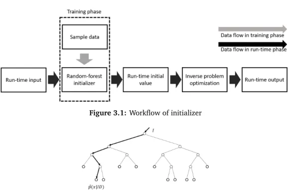
Workflow

As shown in Fig. 5.2, the workflow that builds the initializer includes two phases: training and run-time. In the training phase, we ran a sim-ulation of the motion tracking system to generate as many theory-based samples as possible and make input-output pairs. Then we trained the random-forest with these samples to get a classification model. In the run-time phase for every frame, we put the latest sensor data into the model to predict the output as an initial value to solve the inverse problem. This workflow, which can be applied to all categories of inverse-problem-based tracking systems that need initial values, adds a per-frame initialization to

(25)

Figure 3.1: Workflow of initializer

Figure 3.2: Decision tree in random-forest for parameterx

them. As stated in section 3.1, as long as the predicted initial value has less error than the other methods, the divergence of the optimization process decreases, especially when tracking loss occurs.

Random-Forest

Random-forest, or a random decision forest, is an effective multi-class classifier that consists of multiple decision trees with splits and leaf nodes (Fig. 3.2). Each split node consists of feature f_θ and thresholdτ. To classify input set I, start at the root and repeatedly evaluate Eq. 3.2, branching left or right based on the comparison to thresholdτ. At each leaf node in the tree, the distribution of outputP (X |I D)~ is stored:

f_θ_{(I , x) = d}I(x + u dI(x)) − d I(x + x dI(x) ) (3.2)

The distributions are averaged for all the trees in the forest to give the final distribution, which is the final possibility of this classifier’s output. A random-forest can be effectively trained with a previously described

(26)

algorithm [73].

Random-forest has two main configurable parameters: the depth of the trees and their number, both of which determine the model’s complexity. In practice, we configure these parameters based on the model’s actual performance through experiments. In section 5, we also show an experiment with which we configured the model for our application example.

Sample Acquisition

Collecting training data is sometimes difficult for precise and high-resolution motion tracking systems. In most previous researches, training data were carefully collected through actual use cases, for example, using accurate robot arms for automatic measurements or manual measurements in small intervals of positions (< 5mm) and rotations (10◦) for the entire tracking space since the machine-learning model’s output directly becomes tracking results. However, our initializer does not require such sampling because the random-forest’s output is used as an initial value that only has to be accurate enough for the optimization process. This actually introduces a possible approach to simply acquire massive samples. As Eq. 3.3 describes, the optimization process of 3D motion tracking systems can be generalized to a process that minimizes the objective function. Herexis the tracking result,

M is the measurements, and f (x)calculates the theoretical measurements for specific tracking resultx based on a tracking principle. Therefore, such optimization is seeking theoretical value xso that f (x) = M. Based on this, we use a simulator to enumerate every possiblexto compute corresponding

f (x)and use these combinations as training samples:

(27)

Figure 3.3: Convergence rate of three methods

3.1.2 Evaluation

Convergence

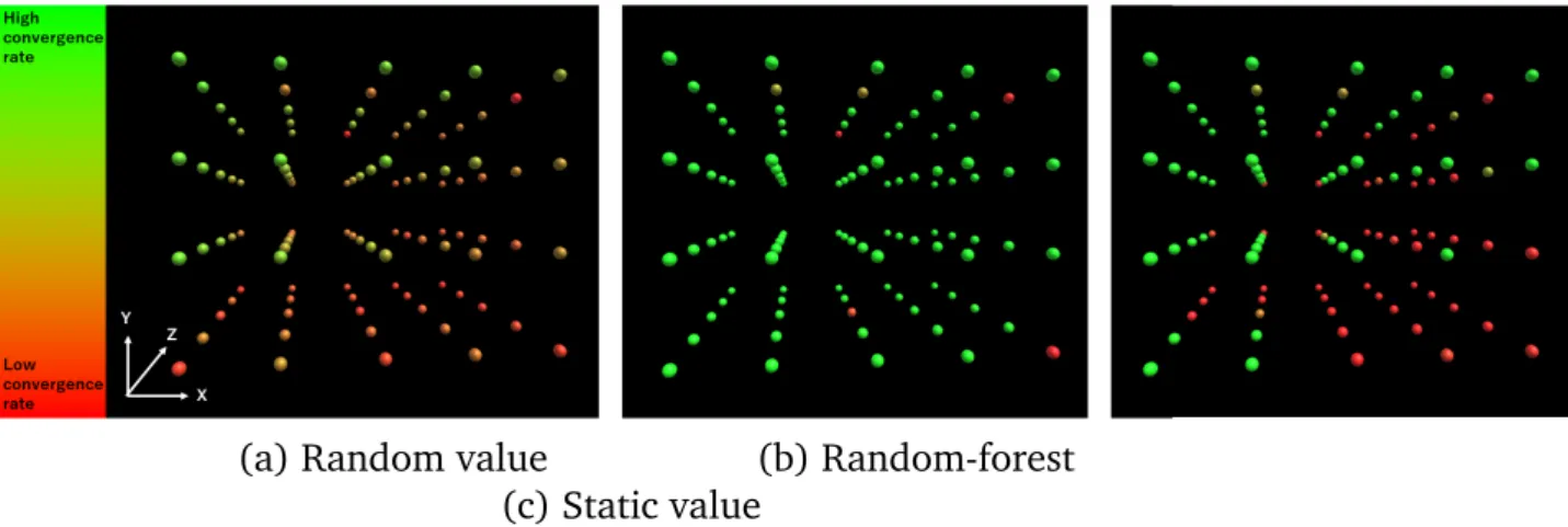
In this section we describe the evaluation of our method that was implemented in IM3D. Through these evaluations we show the benefit of our initializer. Convergence is the most important feature brought to the system by our initializer. Previously without an initializer, when tracking loss occurs, the system has trouble recovering since it cannot find a proper initial value for the optimization process. With our method, the system can ensure a proper initial value, and so the optimization process highly converges when the S/N ratio is acceptable. We experimentally proved this feature and the superiority of our method by comparing our method and two other settings: 1) Always setting the initial value to a static position in the tracking space (x = 0 mm, y = 50 mm, z = 0 mm from the IM3D’s origin), and 2) randomly choosing a value inside the tracking space at every time instance. We chose these two because they are the most common methods used by practical real-time motion tracking systems when tracking loss occurs.

We put a marker at 100 different locations inside the tracking space to uniformly collect data (3 mm, 32 mm, 64 mm, 93 mm, and 122 mm for

x and z axis; 32 mm, 64 mm, 93 mm, and 122 mm for y axis). The real position was measured by a ruler to maintain 1-mm accuracy. The locations

(28)

(a) Random value (b) Random-forest (c) Static value

Figure 3.4: Visualization of convergence rate of three methods

are within one quarter of the whole space because of the symmetry of the pick-up coil layout and evenly distributed inside the space while maintaining differences from typical locations and training samples. We mainly evaluated in several height layers from 32 mm (the lowest height our measurement structure can reach) to 122 mm. We measured flux 100 times in each position and processed the optimization with initial values computed by the three methods. Diverged processes were detected by checking whether the calculated magnetic moment of each process was significantly large. To avoid counting trials in which the processes converged into the local minima of the cost function, we also counted trials as diverged trials when the distance between the calculated position and the actual position was larger than 40 mm.

The convergence rate (t r i al s−di ver g ed_{t r i al s} ) of each method is shown in Fig. 3.3, and the convergence rate of our method significantly exceeds all other methods. Individual results in every specific position are shown in Fig. 3.4. Our initializer has more effective results in almost all the measuring positions, indicating that our initializer can provide better initial values even for areas far from the center of the space. Hence it is more robust. This result also implies that our method will be more effective for other tracking systems with a larger tracking space. Therefore, the initial values predicted by our method are perspective values for computation.

(29)

Figure 3.5: Visualization of prediction accuracy inside space

Prediction

The system with our initializer has same tracking accuracy as a previous work [74] that applied the same principle. However, our random-forest method shows amazing potential in position calculation since the initializer’s output seems very close to the final result. Additionally, we want to confirm that the random-forest yields a prediction that is close to the actual location, so that the inverse problem can be successfully solved. Based on these goals we experimentally demonstrated this feature.

Positional Accuracy We calculated the distances between the initial values predicted by random-forest and the actual positions by using the data we acquired in section 5.1.

The visualized results are shown in Fig. 4.26. The error of each location is mapped in 3D colored dots, and the minimum error (30 mm) is shown as green dots and the maximum error (150 mm) is red dots. Most points are either highly green or highly red. The average prediction error within the tracking space is 35 mm, which is highly satisfactory as an initial value for the inverse problem, since from previous experience an initial value with error less than 70 mm can ensure the convergence in calculation with an acceptable S/N ratio.

(30)

Figure 3.6: Marker (LC coil) on rotating platform

Flux Strength Affect We conducted an additional evaluation with differ-ent rotations and differdiffer-ent numbers of markers. These differdiffer-ent conditions changed the flux sensed by the pick-up coil. We want to evaluate the magnitude of flux with which the initializer can yield a reliable result.

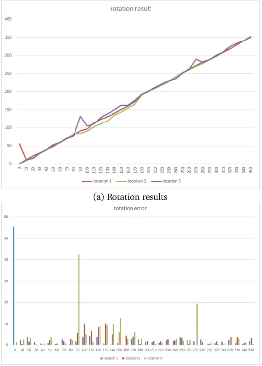
We used a rotating platform (Fig. 3.6) to fix the marker in correspond-ing rotations. In six different locations in the trackcorrespond-ing space, we got the data with both one-marker and fifteen-marker configurations. We defined 90 degrees as a parallel pose to the plane of the pick-up coil array and 0 degrees as a perpendicular pose to the plane. The magnitude of flux decreases when the marker’s pose becomes close to 90 degrees, and the S/N ratio becomes poor.

Fig. 4.5 shows the prediction error in different rotation from various locations, where the error in different locations (coordination represented as X|Y|Z at the top of the graphs) is shown as lines in different colors. These results show that prediction accuracy falls when the flux is reduced, since the accuracy in the larger rotation is lower than that in the smaller ones, and in the same pose, the accuracy in the one-marker configuration is higher than the fifteen-marker configuration. Actually, the IM3D system suffers from this dead-angle problem. When its angle is almost parallel to the pick-up coil array, the LC coil cannot generate any flux, which also caused tracking loss even with proper initial values.

Meta-Parameters of Random-Forest

We also did another experiment to obtain output from our initializer with the measured flux data in experiment in section 5.1 to determine the effects of different parameter configurations. We focused on the estimation success rate, which is defined as the prediction percentage with error smaller

(31)

(a) one-marker configuration result

(b) fifteen-marker configuration result

Figure 3.7: Prediction error in different rotations from different locations

than 50 mm among all the test points. Fig. 3.8(a) shows the success rate when we train the forests with 10-mm interval samples (1.1 million samples) with a maximum tree depth (30 to 70) for four different number of trees (8, 16, 24, 32). This graph shows the results with different combinations of number of trees and maximum depths for each tree. For all the config-urations of different numbers of trees, the success rate reached its highest result with a maximum depth of 60, and with 16 trees the forest reaches its highest rate of 90%.

Fig. 3.8(b) shows the same experiment with 5-mm interval samples (8.8 million samples). Similar to Fig. 3.8(a), it has a peak for the success rate, and more trees increase the success rate.

We also found that the accuracy with 10-mm samples is better than 5 mm by comparing all these results, probably caused by more ambiguity in the excessively massive data samples.

(32)

(a) forests with 10 mm interval training samples

(b) forests with 5 mm interval training samples

Figure 3.8: Success rate with meta-parameters (i.e., maximum depth of

trees and number of trees)

Figure 3.9: Speed (in FPS) decreases when markers (LC coils) increase

Performance

For a real-time motion tracking system, since its computational speed’s performance must be ensured, we also did such experiments. We mainly tested the speed of the entire process (our initializer and the optimization process) and the initializer’s speed itself.

For the random-forest performance, we simply ran the random-forest evaluation 1000 times and checked the time cost. Each prediction call cost 1 millisecond, which barely affected the entire system’s performance.

(33)

number of markers ranging from 1 to 15, ran it for 100 seconds, and tracked all the used markers. The system provided high-tracking speed close to 60 Hz for a marker. When tracking with up to 15 different markers, it can still maintain a speed over 30 Hz (Fig. 4.6). The speed reduction is caused by the increase of overhead, other than introduced by our initializer.

3.1.3 Discussion

Due to resource limitations, we only implemented our method on the system based on the tracking priciple. However, as mentioned in section 3, it can generally be applied to other optimization-based tracking systems. As in these systems, since simulation is easier than solving the inverse problem, massive training samples can be easily obtained from the simulation. For example, for camera-based optical tracking systems, the simulation input can be rendered as images with specific camera-marker configuration, and for magnetic tracking systems, the simulation input can be theoretical values with specific marker locations and rotations.

The evaluation results proved that this method adds robustness to 3D motion tracking systems. Since interactive techniques always require continuous tracking results for continuous interaction, our method, although not directly, will also improve the experience of 3D motion-based interactive techniques.

We chose to experiment with a random-forest rather than other data-driven methods, such as a deep neural network (DNN) or the Gaussian process. Actually, we tested these methods with the same input-output strategy and training data through preliminary research. However, none of these methods yielded satisfactory results, perhaps due to the complexity and the ambiguity of such inverse problems or the model’s complexity during run-time. On the other hand, without yielding very accurate results, random-forest constantly gave acceptable predictions very quickly; we choose it because it is a fast and accurate initializer.

Regarding the run-time phase, random-forest works like lookup tables, which only search from existing data to find the best match. Since we can

(34)

generate a very large database using the Biot-Savart law without much effort, such a method might effectively get close output. Based on this difference, perhaps other similar methods (for instance, KD trees) might be successful, although further experiments are needed.

Our evaluation shows that our initializer itself is so fast that there is almost no effect on the system’s cost. This leaves space for further improvements, such as filters or regression.

3.2 DNN-based Optimization Solver

It is possible to use deep-learning to construct a data-driven solver instead of Gauss-Newton method to solve the optimization problem for the tracking system. In this way, since we anticipate high-speed computation without any initial values, the computation becomes robust. In this sec-tion, the detail of this solver, including implementation and evaluasec-tion, is provided.

Preparing the Training Data

In this section, we describe the process of preparing the training data for our method.

Recall that in the proposed magnetic tracking system, we have

B (C) = µ0 4π ½ − M krk3+ 3( M · r )r krk5 ¾ · v (3.4)

where M is the magnetic moment of the LC coil whose orientation corre-sponds to the orientation of the LC coil represented by θ and φ and its amplitude by scalar M,vis a unit vector in the direction of the flux sensor, andris the location of the LC coil. Since each LC coil has a unique induction frequency, even though the flux sensors can only measure the sum of the induced voltage from different LC coils, the contribution of each LC coil can be extracted using fast Fourier transform (FFT).

(35)

Using Eq. (3.4) and the induced voltage at each sensor, spatial configu-rationC of each LC coil can be computed. [74] solvedCnumerically by the Gauss-Newton method for which the voltages from at least six sensors are needed, but the solver requires a good initial estimate ofC. Also the compu-tation does not converge well when the induced voltages of the sensors are small.

Instead of collecting actual marker-sensor data pairs from a motion-tracking system, we employ the theoretical simulation data using Biot-Savart’s law. With Eq. (3.4), we can calculate voltage B = (B1, ..., BN)

gen-erated by an LC coil marker at configurationC, whereN is the number of flux sensors. A large number of(B, C)pairs can then be obtained within the defined capture volume for training.

When learning the mapping from sensor valuesBto the configurations of LC coil marker C, instead of usingB as is, we perform normalization and

use the normalized data_Bˆ _{for training where}_{B = B/max(abs(max(B)), abs(mi n(B)))}ˆ _.

This is because the raw sensor data change in an unpredictable manner due to the varying induction intensity, i.e., the amplitude of the magnet moment of the LC coil as a source (scalar M described in 4.3.2), among different LC coils in different 3D configurations. On the other hand, the Biot-Savart law (Eq. (3.4)) indicates that the ratio between any two sensor fluxes (e.g.,

B1 andB5) stays the same whenBvaries. Thus usingBˆ is more stable and

provides good mapping.

Network Structure

We use a feedforward neural network to regress the measurements at flux sensors to the spatial configurations of the markers (LC coils). Our network is composed of several fully connected layers, each of which is followed by RELU activation functions:

Φ(X;β) = W4RELU(W3RELU(W2

(36)

whereXis the input vector andβ = (W0, b0, ..., W4, b4)are the network weights

and biases. Here we use four fully connected layers with hidden unit numbers of 1024, 2048, 4096, and 1024.

3.2.1 Training

To train the network, we minimize the following loss function based on the mean square error (MSE) using stochastic gradient descent:

Loss = kΦ(X;β) −C k2+ γ|β| (3.6) whereC is the ground-truth configuration of the marker and the second term is the L2 regularization term. In our work γ is set to 0.0005. The system is implemented in Keras [75] with Tensorflow [76], and we use Adam solver [77] to speed up the convergence.

The training takes two hours on a computer with two NVIDIA GeForce GTX 1080ti GPUs to reach a loss less than 0.0001 using approximately 180,000,000 pairs of random simulation samples.

3.2.2 Discussion

The DNN-based solver can be regarded as an extension to the idea proposed in Section 3.1, i.e., use machine-learning approach to solve an optimization problem. In this specific case, DNN shows good precision, however the question whether it can be applied in other cases remains to be explored. This research shows a possible practice, however, for other similar applications that training data can be collected via simulation. Con-sidering the fact that manual data acquisition is extremely labor-heavy, the simulation approach is actually important. In our experience, it takes 3 hours if we manually collect 200,000 samples, while simulation only takes 2 minutes. This is also valid because for an inverse problem the goal is to match the actual measured data to one that is obtained through theoretical computation, therefore simulation data does not invalidate the process.

(37)

Figure 3.10: Workflow of structure-aware temporal bilateral filter

3.3 Structure-aware Bilateral Temporal Filter

In not only the tracking principle but also the DNN optimization solver, the output requires further filtering because artifacts exist due to the back-ground and hardware noise, regression ambiguity, and the dead-angle problem. Actually, such artifacts exist in the naive implementation of the tracking principle and prevent it from satisfactorily capturing the motion. Dead-angle configuration can also cause the complete loss of the tracking result for a short period of time.

In this section, we describe how we overcome these issues by propos-ing a structure-aware temporal bilateral filter (SATBF) that computes the weighting of time-series data based on the sensor information. This filter-ing method effectively reconstructs the captured motion data, because the high-dimensional sensor output functions well as a weighting factor for computing the weights of the surrounding configurations in a time window.

3.3.1 Algorithm

We describe the SATBF algorithm within the context of our specific problem; however, SATBF can be applied to any nonlinear system. SATBF’s workflow is demonstrated in Fig. 3.10. Our structure-aware bilateral filter is a weighted average filter with a time window of size N. For time instance

i, letsn (n = −N₂, ...,N₂)be the state vector within the time window, wheresn

(38)

the 3D configuration of the marker predicted by the DNN in our case), and sensor data_Bˆ_: _s_n_{= t}_n_{, r}_n_{, ˆ}_B_n_.

Our SATBF computes the filtered configuration as follows:

Ci= 1 K X n rne−α d (i ,n) ρ _e−β|ti −tn |σ (3.7) K =X n e−α d (i ,n) ρ _e−β|ti −tn |_σ _(3.8)

whereCi is the filtered configuration.

ρ,σ, which are standard deviations of the Gaussians, are set to 0.2 and 1. α,β are weighting parameters set to 2 and 1, and d (i , n) is a distance function that computes the weighting of frame n based on the sensor values defined as follows:

d (i , n) = k ˆBi− ˆBnk (3.9)

Eq. (3.7) is a bilateral filter whose weighting is defined based on the sim-ilarity of the sensor values and the temporal closeness. It also resembles the NLM filter where the patch similarity is used for the weighting. Using sensor values for the distance function produces much better results than when only configuration valuesrn are used for filtering. See Section 3.3.3

for a comparison. .

3.3.2 Integration with the tracking principle

When computing the distance function with Eq. (3.9), we use nor-malized sensor values _Bˆ _{to eliminate the effect of the varying magnetic}

moment.

We also preprocess the data sequence to recognize and remove the corrupted frames. The frames are evaluated based on the temporal variation of configurationrn with respect to the variation in sensor dataBˆ.

In our pilot study, we found that the dead-angle problem occurs fre-quently and causes short sequences of corrupted frames. Therefore we chose

(39)

(a) pendulum move (b) circular move (c) line move by gear

Figure 3.11: Configurations using robot arm for filter evaluation

experi-ments. Marker is shown within red rectangles.

a window size of 20 for the filter to ensure that available neighbors exist.

3.3.3 Evaluation

We now compare the results computed using our structure-aware tem-poral bilateral filter (SATBF) with other alternatives, including the Un-scented Kalman Filter (UKF) [33], one of the most widely used general-purpose filters in real-time motion-tracking systems, a bilateral filter with a distance function based on the marker configuration (BF-conf-dis), an NLM filter [39], and a temporal convolutional filter (TCF) trained with data collected by moving the sensors in the capture domain [78]. The temporal convolution filter is composed of three layers with 32, 64, 128 feature maps in each layer. The filter width is set to 2×2 and trained with 500 minutes of marker data (sampled in 30 Hz).

As shown in Fig. 3.11, we utilized a robot arm to accurately and repeat-edly move one marker in certain patterns and record its motion. For the pattern shown in Fig. 3.11(a), we used the robot arm to move a pendulum with a marker attached perpendicularly to the robot’s stick. When the robot arm moves, the marker passes the lowest point with a horizontal pose, and therefore the flux sensor can only sense very low flux signals, causing track-ing loss. For the pattern shown in Fig. 3.11(b), the marker is horizontally attached to a stick (parallel to the flux sensor plane) and moved circularly in a horizontal plane. The flux sensors constantly sense the low flux signals due to the marker’s pose, causing a noisy tracking result. In the pattern in

(40)

Fig. 3.11(c), we attached the marker to a gear and used the robot arm to drive it forward/backward to rotate the gear along the rail (from the top, the movement resembles a straight line). Again, when the marker rotates to a horizontal pose the sensors can only detect very low flux signals, resulting in tracking loss.

The results of this experiment are shown in Fig. 3.12, 3.13, 3.14. DNN’s raw output is shown as blue dots in each graph, and the expected tracking loss from the low sensed flux signal can be observed in each of them. The tracking loss obviously causes non-Gaussian noise (i.e., non-white). Such noise is very difficult for general filtering methods to process.

As shown in Fig. 3.12, Fig. 3.13, Fig. 3.14, our filter (SATBF, 1st items of the figures) stably follows the original curves, although the raw outputs from the DNN are rather noisy and unstable in some regions. UKF fails to filter such noise in many instances (2nd items of the figures). Although the BF-conf-dis and NLM results are much more stable, they sometimes fail to converge at the correct location due to singularities (see 3rd and 4th items in the figures). This problem can be attributed to the fact that neither of these methods uses the sensor data to compute the weighting since the configurations are rather random near the dead angles due to the ambiguity of the regression and environment noise. The TCF results are rather disappointing (5th items of the figures), given that the system is learning from raw trajectory data with ground truth from the optical motion capture data. This failure could be attributed to the ambiguity of signal when the marker is near a dead-angle configurations that harms the training, since many movements pass through the dead angles when the training data are captured.

3.3.4 Discussion

The SATBF works robustly in our experimental results. Its key idea is to compute the state distance in the sensor measurement spaces rather than in the marker configuration spaces. We found that this approach significantly stabilized the trajectories and increases our system’s viability for practical

(41)

SATBF UKF

BF-conf-dis NLM

TCF

Figure 3.12: Raw and filtered results of a tracked LC coil. Trajectories

in raw DNN output (blue) are compared with different filtering results (orange).

(42)

SATBF UKF

BF-conf-dis NLM

TCF

(43)

SATBF UKF

BF-conf-dis NLM

TCF

(44)

applications.

The following is one description for success; The noise in the sensor space can be well described by Gaussians, although its nonlinear transfor-mation through the DNN can no longer be described by Gaussians. Since bilateral filters only assume noise that can be described by Gaussian dis-tributions, it will be difficult to filter the noise only using the data in the configuration space.

3.4 Summary

In this chapter, 3 major processing methods, which can be used to solve the limitations of the tracking principle, are proposed. While random forest can be integrated with the Gauss-Newton solver to solve the initialization problem, the DNN can solve the initialization problem as well as increase the computation speed. Anothe benefit of DNN is the flexibility of sensor layout, which also increases the potential of the system for variety of applications. These two methods can be used in different scenarios. SABTF can solves the dead-angle problem of the tracking principle to ensure continuous tracking without losing frames. In the next chapter, the integration of these methods to the tracking system is introduced. With different integration, systems with different features can be implemented. The evaluation will then be executed together with the actual hardware.

(45)

Chapter 4 Prototypes

This chapter introduces 3 iterations of the system prototype: IM3D, IM6D, and IM6D+. The progress of iterations shows not only the result of this research, but also the baseline of the tracking principle (hence the reason why it needs improvement). IM6D and IM3D+ are different solutions based on different approaches, therefore they have different consideration of trade-offs and can be used in tasks with different requirements.

4.1 IM3D: Magnetic Motion Tracking System

for Dexterous 3D Interactions

4.1.1 Overview

IM3D (shown in Fig. 4.1) is our first hardware implementation based on the tracking principle. By incorporating high performance computing hardware and parallel computation scheme, it achieves real-time tracking. However, since it’s a naive implementation, it inherits all the limitations of the tracking principle.

(46)

Figure 4.1: The hardware setup of IM3D

Hardware setup

To create a semi-sphere tracking area with a 150-mm radius, the system uses 32 pick-up coils with a 15-mm radius and 60-mm intervals between the coils. The application scenario uses a plane layout with a driving coil set at the same horizontal plane, an AD converter set (PXIe-1075, NI Ltd.), an amplifier (HSA4011, NF Ltd.) + function generator (PXIe-6124, NI Ltd.) for generating the signals, and a conventional computer (Xeon E3×2, Intel Ltd., 16G RAM, Titan Black×1, NVidia Ltd.) for multi-thread computation. System and layout images of the pick-up coils are shown in Fig. 4.1.

The system can simultaneously track a maximum of 15 LC coils (i.e., five markers) at 30 fps. The coils’ Ni-Zn ferrite cores are 4-mm radius, 15-mm long cylinders. The turns of the Polyester Enameled Copper Wire (PEW) for each LC coil range from 100 to 600 (details in Table 4.1), making their resonant frequencies different for unique identifications (Fig. 4.2). Fig. 4.3 shows the LC coil and designs of markers. A transparent heat-shrink tube covering protects the LC coil, which weighs about 1 g. We used a 3D printer with high accuracy to produce the markers with a cage design. The rings are about the size of human fingers, and the radius of the tube used to fix the LC coils is kept to the minimum.

(47)

Table 4.1: Maker Specifications

Peak Re-Marker Coil turn Condenser sonance

Fre-ID (pF) quencies (kHz) Z 600 1500 61.5–62.2 A 600 680 88.9–89.9 B 500 560 119.0–120.2 C 384 560 153.3–154.8 D 350 470 181.1–182.9 E 295 470 208.5–210.4 F 247 560 242.2–244.6 G 194 680 269.8–272.3 H 193 560 302.4–305.1 I 186 470 328.7–331.6 J 189 390 359.7–362.8 K 142 680 388.3–391.8 L 146 560 419.7–423.4 M 147 390 445.5–449.4 N 105 820 482.3–486.3

Figure 4.2: Different resonant frequencies for different markers

(a) LC coil (b) cube (c) arch (d) dodecahedron (e) ring

(48)

4.1.2 Features

IM3D, as the initial implementation based on the novel magnetic track-ing principle, serves several purposes. First, . The feature of this system includes:

• Occlusion-free tracking • High accuracy

• Real-time speed

• Up to 15 markers with unique IDs • Lightweight markers

4.1.3 Evaluation

In this section the performance and specifications of IM3D is evaluated to give details of the features introduced in Sec. 4.1.2.

Static Accuracy

Our static accuracy experiment focuses on the accuracy of each single LC coil because the 6-DOF markers’ accuracies completely rely on its accuracy. We put an LC coil at different locations inside the designed workspace using a 3-axis mechanical position controller with a high-accuracy laser range finder and took 100 samples to investigate its performance. We used a common coordinate system in which XZ shows a plane of the pick-up coil array and Y is vertical to this plane, where the origin is the center of the pick-up coil array’s plane. This evaluation only occupies a quarter of the whole tracking space, and since the layout of pick-up coils is symmetrical, the remaining part will yield exactly the same results.

As shown in Fig. 4.26, the results imply two interesting points. First, the tracking error, defined as the variance of the result in each location, appears to be low. The results also show that, even at the edge of the designed tracking space (a 150-mm radius semi-sphere), the original error

(49)

(a) Raw results on XY plane (b) Regression results on XY plane

(c) Raw results on XZ plane (d) Regression results on XZ plane

(50)

between the raw data and the real position (white rectangles) remains less than 5 mm as shown in Fig. 4.26(a)(c). This result proves that our system is feasible for dexterous-motion-tracking tasks. Second, the tracking result shows a bias approaching the origin. To prove this, we continued to take samples out of the designed tracking space, and the result matches our expectation. This can be explained by signal attenuation due to the distance, and such non-uniformity of accuracy actually exists in almost every tracking system. We believe that this bias can be corrected by regression methods, and so we did a machine-learning-based regression with limited samples. We trained a simple 3-layer artificial neural network (ANN) with half of the tracking results and later used it to process the rest. As shown in Fig. 4.26(b)(d), the corrected result (blue points) is satisfactory, since within the tracking space, the distance between the actual and computed locations is as close as 1 mm. This method can be easily applied to a larger scale of samples, given the system’s ability to correct the bias of the coils in any pose.

Similarly, rotational accuracy of single LC coil is measured by rotating the coil around a axis using a rotatable mechanical structure set on the plane of pick-up coils. Results obtained from three typical locations in the tracking space is shown in Fig. 4.5. Here, average error is 2.21 degrees in φ and 1.89 degrees inθ; however, larger errors can be seen around the dead-angle (90 and 270 degree) where the axis of the LC coil becomes closer to parallel to the pick-up coil array. Our marker design with three LC coils solves this problem because at least one LC coil is always available; thus the system can reduce the rotational error.

Speed

We experimentally investigated the tracking speed of our system. We ran a graphics application that indicated the marker poses and took 30-second bits of speed data during a normal tracking task to randomly track the moving fingers.

(51)

(a) Rotation results

(b) Rotation error

(52)

Figure 4.6: FPS Evaluation

15 LC coils), our system is still faster than 30 Hz, and variance exists due to the different time cost for convergence in different situations. The number of markers only slightly affects the speed of the system. This is because our computation structure handles each part of the computation in different computing units (i.e., CPU and GPU) and the system’s hardware has the potential to support up to ten markers (with 30 LC coils) without decreasing the speed.

4.1.4 Limitations

IM3D is relatively a naive implementation of the magnetic tracking principle, therefore it naturally inherits the systematic limitations. The first and most important limitation is called the “dead-angle problem”. The flux of the driving signal (the magnetic field) has certain direction, therefore, once the marker is perpendicular to the driving signal, it fails to get induced thus cannot generate any resonant signal, concequently the marker cannot be tracked.

track metal objects. However, metallic objects in the environment will not affect the tracking result as long as they do not get very close to the marker or occlude it from flux sensors. LC coils generate resonant magnetic fields at a specific frequency because a random metallic object rarely generates a magnetic field at the same one. Therefore the signals do not overlap.

(53)

4.2 IM6D: Magnetic Tracking System with

6-DOF Passive Markers for Dexterous 3D

Interaction and Motion

4.2.1 Overview

The tracking principle in previous system indicates an important and serious problem: unreliable coil tracking. The computation of the inverse problem requires a proper initial value and a strong enough resonant flux; however, it is impossible for the principle to ensure that these two factors are appropriate. During tracking, once the LC coil is in a range of pose, it cannot be driven. This is called the dead-angle problem. Actually, this happens when the axis of the LC coil falls within ±15 degrees against the plane of the pick-up coil array, and it is quite usual during practical tasks. In such a pose, the position and orientation of the LC coil cannot be properly computed. As a consequence, the initial value of the next time instant is corrupted, and the system loses the ability to track the LC coil. This critical problem prevents the principle from succeeding in practical long-term use. To solve this problem, we propose a geometrical approach that contains three LC coils with different poses in one marker, in which relative positions and orientations of the three LC coils are known. We define the situation of being driven as “available” and the other situation as “unavailable.” In our design, the system ensures that in any situation, for any marker, at least one LC coil is available. Thus, it gains tracking continuity. Another ability gained through this design is 6-DOF tracking, since generally in practical use two or more LC coils are available in one marker. The information of two incomplete 5-DOF LC coils helps to indicate the 6-DOF pose of the marker, and it is expected to improve the tracking accuracy.

Here, we simplify the shape of the marker into a rigid cube as shown in Fig. 4.7; however, it can be applied to any shape of LC coil combinations. The system first select one of the three LC coils which has the strongest resonant flux as the “main” (assume to be LC coil A in this figure). This LC

東北大学機関リポジトリTOUR

Practical Processing Techniques for Magnetic

3D Motion Tracking

著者

黄 佳維

学位授与機関

Tohoku University

学位授与番号

11301甲第19343号

URL

http://hdl.handle.net/10097/00130233

TOHOKU UNIVERSITY

SENDAI, JAPAN

P

RACTICAL PROCESSING TECHNIQUES FOR

MAGNETIC

3D

MOTION TRACKING

A dissertation submitted in conformity with the requirements for

the degree of Doctor of Philosophy

R

I

E

C

G

S

I

S

by

Jiawei HUANG

Supervisor

Yoshifumi KITAMURA, Professor

Abstract

Contents

Chapter 1

Introduction

1.1

Background

1.2

Magnetic Tracking Principle

1.3

Objective

1.3.1

Initialization

1.3.2

Speed

1.3.3

Dead-angle

1.3.4

Flexibility

1.3.5

Application

1.4

Contribution

1.5

Overview

Chapter 2

Related work

2.1

Motion Tracking Systems

2.2

Data-driven Methods

2.3

Filtering

2.4

Dexterous Motion Capture

2.5

Human-Computer Interaction

2.5.1

Finger-based Dexterous Interaction

Chapter 3

Processing Techniques

3.1

Random Forest-based Initializer

3.1.1

Method

3.1.2

Evaluation

3.1.3

Discussion

黄佳維