JAIST Repository: Investigation of Modal Logics with Application to Agent Communication [課題研究報告書]

(1)

JAIST Repository

https://dspace.jaist.ac.jp/

Title Investigation of Modal Logics with Application to Agent Communication [課題研究報告書]

Author(s) Arai, Norihiro Citation

Issue Date 2014-03

Type Thesis or Dissertation Text version author

URL http://hdl.handle.net/10119/12029 Rights

(2)

Investigation of Modal Logics with Application to

Agent Communication

By Norihiro Arai

A project paper submitted to

School of Information Science,

Japan Advanced Institute of Science and Technology,

in partial fulfillment of the requirements

for the degree of

Master of Information Science

Graduate Program in Information Science

Written under the direction of

Professor Hajime Ishihara

(3)

Investigation of Modal Logics with Application to

Agent Communication

By Norihiro Arai (1210003)

A project paper submitted to

School of Information Science,

Japan Advanced Institute of Science and Technology,

in partial fulfillment of the requirements

for the degree of

Master of Information Science

Graduate Program in Information Science

Written under the direction of

Professor Hajime Ishihara

and approved by

Professor Hajime Ishihara

Associate Professor Kazuhiro Ogata

Professor Satoshi Tojo

February, 2014 (Submitted)

(4)

Abstract

This paper presents basic knowledge of modal logics as a preliminary stage of studying epistemic logic. Modal logic is a logic based on classical logic. The most important characteristic of this logic is that it could deal with necessity (“it is necessary”) and probability (“it is possible”), often represented by the symbol □ and ♢, respectively. A modern modal logic is created by Lewis(1932)[1]. In the early 1960s, Kripke introduce a semantics called “Kripke sematics”, which is widely used on modal logic today[2][3][4]. It is well-known that, when we denote“a person A knows φ”and“a person A believe φ” by“KAφ”and“BAφ”, respectively, there is a lot of common properties between K or B

and□. The logic which deal with knowledge and belief is called epistemic logic, and there are lots of researches which aim to represent agent communication with this logic itself or some variations of this logic, where agent communication is the communication between multi-agent environment: an exchange of messages on Facebook is one of the example of agent communication, which is studied by K. Sano and S. Tojo(2013)[6]. Epistemic logic is based on modal logic, as mentioned above, thus it is important to understand basic knowledge of modal logic before studying agent communication.

In the first part of this thesis, we define the syntax of modal logic K: we denote the propositional variables by the lower-case letters, possibly with subscripts of superscripts; the lower-case Greek letters are reserved as formulas, and capital Greek letters are used for denoting sets of formulas. Syntactically, the only diﬀerence is that one unary symbol □ is added to Cl; a formula of the form ♢φ is defined as the abbreviation of ¬(□(¬φ)).

Second, we see Kripke semantics and its basic properties. One of the strong point of this semantics is that the model in this semantics could be drawn in graph, which could be intuitively understood without deep mathematical knowledge. A model of this semantics is a triple ⟨W, R, V⟩, where W is a non-empty set, R is an arbitrary binary relation on W , and V is an arbitrary map from VarML to P(W ). A pair ⟨W, R⟩ is called a frame and so a model of Kripke semantics could be also regarded as a pair of a frame and a valuation. After that, we see the truth-relation of this semantics, which is natural extension of that of classical logic, and some properties of modal symbols /Box and ♢. We also see a few well-known operations for models which never change the truth-value of each formula. The operations we check are called generation and reduction: generation is defined by taking a generated submodel; and reduction is defined by taking a map which is called p-morphism. We could consider many classes of frames with their property, and the property of those classes are correspond to specific modal formula. We see some major classes and those corresponding formulas: the class of reflexive, transitive, symmetric and serial frames are correspond to the formula□p → p, □p → □□p, p → □♢p and □p → ♢p, respectively. There is a great tool, which is called Hintikka system, to construct a counter model. Hintikka system is a pair h = ⟨T, S⟩ where T is a set of a pair t = (Γ, ∆) of formulas, which is called tableau, with some restrictions and S a binary relation on T . With this system, we can also infer the decidability of this semantics.

(5)

Third, we introduce a Hilbert-style deduction system, which is called calculus K. The only diﬀerence between classical Hilbert-style system is that there is an additional axiom □(φ → ψ) → (□φ → □ψ) and inference rule RN: given a formula φ, we infer □φ. As calculs K is based on classical Hilbert-style system, a formula which is valid in classical logic is also valid in this system. There is a famous theorem in classical logic, which is called deduction theorem, i.e., Γ∪ φ ⊢ ψ ⇒ Γ ⊢ φ → ψ. With some restrictions to RN, we can formulate deduction theorem for modal logic as it was formulated for classical and intuitionistic logic, however, the formulation of this theorem for modal logic is a bit diﬀerent. Calculus K is sound and complete with respect to Kripke semantics of course. On proving the completeness, we use Hintikka system and a specific construction of tableaux. There could be many extensions of logic K, and soundness and completeness theorem alos holds for some of them. On provng these theorem, canonical models and filtration are useful; we briefly see these techniques.

Forth and the last, we briefly see another semantics which is called algebraic semantics. There are lots of semantics other than Kripke semantics, and algebraic semantics is one of them. As algebraic semantics is based on algebra and algebra is very abstract, this semantics could be possibly apply to many fields.

Almost all of the contents in this thesis are mainly based on A. Chagrov and M. Zakharyaschev(1997)[7].

(6)

Acknowledgements

First of all, I would like to express my gratitude to my supervisor, professor Hajime Ishi-hara, for his great support over the last two years. Though I hadn’t studied mathematics before belonging to his laboratory, he has been tolerant and supportive to let me know what a logic is. Without his encouragement, this thesis would not have been possible.

I would also like to thank associate professor Kazuhiro Ogata and professor Satoshi Tojo for their constructive comments and warm encouragement.

Assistant professor Takako Nemoto gives me many insightful comments and suggestions for this thesis. Her meticulous comments were an enormous help to me.

Lastly, I thank the member of Ishihara laboratory and assistant professor Katsuhiko Sano for their advice, and my family for their support and encouragement.

(8)

Chapter 1 Introduction

The inference we often do in our daily life is based on the imperfect knowledge and information about the situation we are facing. The knowledge and information we have shall change every moment, and the truth of them could be overthrown in the future. Moreover, the consequence of our inference directly links to our action so that it is required to infer something, even if the consequence is not satisfying. It is not too much to say that our daily inference is vague, and this is why the importance of a logic available to deal with such a vagueness is growing in the field of agent communication.

Modal logic is a logic which could deal with such a vagueness. In the sense of mathemat-ics, a modal logic is the logic which two connectives □ and ♢ are added to classical logic: □ and ♢ are often used to represent “it is necessary” and “it is possible”, respectively. A modern modal logic is created by Lewis(1932)[1]. In the early 1960s, Kripke intro-duce a semantics called “Kripke sematics”, which is widely used on modal logic[2][3][4]. It is well-known that, when we denote “a person A knows φ” and “a person A believe

φ” by “KAφ” and “BAφ”, respectively, there is a lot of common properties between K

or B and □. The logic which deal with knowledge and belief is called epistemic logic. Recently, many researches are done which aim to represent agent communication using epistemic logic itself or some variations of this logic. S. Tojo(2012)[5] uses a variation of epistemic logic to analyze how the court correct his/her knowledge in a trial. K. Sano and S. Tojo(2013)[6] represent agent communication with a communication channel.

This thesis presents basic knowledge of modal logics as a preliminary stage of studying epistemic logic. First we define the syntax. Second we see one of the major semantics on modal logic, i.e. Kripke semantics and its basic properties. After that, we introduce a Hilbert-style calculus, which is called calculus K, and prove the soundness and com-pleteness theorem. We also see another semantics, algebraic semantics to deepen our understanding. In the end, we interrelate a modal logic to epistemic logic, which is often used on researching agent communication. The contents of this thesis are mainly based on A.Chagrov and M. Zakharyaschev(1997)[7].

(9)

Chapter 2 Kripke Semantics

2.1 Preliminaries

In this section, we define syntax and some terms of our logic. First of all, we define the syntax.

Definition 2.1.1 (Language ML). Fix the propositional modal language ML whose

primitive symbols (alphabets) are:

• the propositional variables p0, p1, . . . ;

• the propositional constant ⊥ (falsehood);

• the propositional connectives ∧ (conjunction), ∨ (disjunction), → (implication), □ (necessity);

• the punctuation marks ( and ),

and the formulas of ML (or ML-formulas, or simply formulas if ML is understood) are defined inductively as

• all the variables in ML and the constant ⊥ are atomic ML formulas;

• if φ and ψ are ML-formulas then (φ ∧ ψ), (φ ∨ ψ), (φ → ψ) and (□ψ) are also ML-formulas;

• a sequence of primitive symbols in ML is a formula iﬀ this follows from the two preceding items.

We will denote propositional variables by the lower-case letters p, q, r, possibly with subscripts or superscripts; the lower-case Greek letters φ, ψ, χ and may be some others are reserved as formulas, and capital Greek letters like Γ, ∆, Σ are used for denoting sets of formulas. There are countably many propositional variables, however, other symbols are countable. The set of all variables in ML is denoted by VarML. Unless otherwise indicated, we will assume VarML to be countable. The set of all formulas in ML is denoted by ForML.

(10)

Definition 2.1.2 (Subformula). Let φ and ψ be formulas. We say that a formula χ is a

subformula of φ if one of the following is satisfied: • χ ≡ φ;

• φ ≡ ψ ⊙ χ or φ ≡ χ ⊙ ψ, where ⊙ ∈ {∧, ∨, →}; • φ ≡ □χ;

• χ is a subformula of ψ and ψ is a subformula of φ.

We denote the set of all subformulas of φ and all variables in φ by Subφ and Varφ, respectively.

The propositional connectives ¬ (negation), ↔ (equivalence), ♢ (probability) and the constant ⊤ (truth) can be defined as abbreviations:

(¬φ) = (φ → ⊥),

(φ ↔ ψ) = (φ → ψ) ∧ (ψ → φ), (♢φ) = (¬(□(¬φ))),

⊤ = (⊥ → ⊥).

We shall use the following standard conventions on representation of formulas: we assume

¬, □, and ♢ connect stronger than ∧ and ∨, which is stronger than → and ↔, and omits

those brackets which we can recover without any confusion. We shall write φ1,∧ · · · ∧ φn

or ∧₁_≤i≤nφi instead of (· · · ((φ1 ∧ φ2)∧ φ3)∧ · · · ∧ φn) and φ1,∨ · · · ∨ φn or

∨ 1≤i≤nφi instead of (· · · ((φ1∨φ2)∨φ3)∨· · ·∨φn); ∨ i∈∅φi and ∧

i∈∅φimean⊥ and ⊤, respectively.

2.2 Possible World Semantics

Next, we define the semantics of modal logics. We use possible world semantics, one of the most major semantics in modal logics.

Definition 2.2.1 (Modal Kripke frame). A modal Kripke frame F is a pair⟨W, R⟩ where

• W is a non-empty set;

• R is an arbitrary binary relation on W .

Elements of W are called worlds or points. Let x, y ∈ W . If xRy, we say that y is accessible from x, x sees y, y is a successor of x, x is a predecessor of y, y ∈ x ↑ or x∈ y ↓.

Definition 2.2.2 (Valuation). Let F =⟨W, R⟩. A valuation V on F is a map such that

V : VarML → P(W ).

Definition 2.2.3 (Kripke model). A Kripke model of ML is a pair M = ⟨F, V⟩ where

(11)

Definition 2.2.4 (Truth-relation). Let F =⟨W, R⟩ be a modal frame, x be a point in W ,

(M, x)|= □ψ iﬀ (M, y)|= ψ for all y ∈ W such that xRy,

and so

(M, x)|= ¬ψ iﬀ (M, x)⊭ ψ,

(M, x)|= ♢ψ iﬀ (M, y)|= ψ for some y ∈ W such that xRy.

Now let us see some basic properties of Kripke semantics.

Definition 2.2.5 (Accessibility). Let F = ⟨W, R⟩ be a modal frame and x, y ∈ W . Say

that y is accessible from x by n≥ 0 steps and denote xRn_{y or y}_{∈ x ↑}n _{or x}_{∈ y ↓}

n if there

exists (not necessarily distinct) points z1, . . . , zn−1 ∈ W such that xRz1R· · · Rzn−1Ry.

Note that xR0y, y ∈ x ↑0 and x∈ y ↓0 are understood as x = y. Proposition 2.2.6. For every n≥ 0,

(a) (M, x)|= □nψ iﬀ ∀y ∈ x ↑n[(M, y)|= ψ],

(b) (M, x)|= ♢n_ψ _iﬀ _{∃y ∈ x ↑}n_{[(M, y)}_{|= ψ].}

Proof. Let M =⟨F, V⟩. We prove these two by induction on n.

(a) (⇒)

n = 0

Suppose that (M, x)|= □0_{ψ. Fix any y} _{∈ W such that y ∈ x ↑}0_{. Our goal is}

to show (M, y)|= ψ, and this is obvious since y ∈ x ↑0 _{means y = x.}

n = k + 1 (k≥ 0)

Suppose that (M, x)|= □k+1ψ. Fix any y ∈ W such that y ∈ x ↑k+1. Our goal is to show (M, y)|= ψ. By the assumption, we have (M, x) |= □k(□ψ) and so, by the induction hypothesis,∀z ∈ x ↑k_{[(M, z)} _{|= □ψ] holds. Since y ∈ x ↑}k+1_,

there is a point z∈ W such that z ∈ x ↑k and zRy. Therefore we have (M, z)|= □ψ

⇔∀y ∈ W [zRy ⇒ (M, y) |= ψ],

(12)

(⇐)

n = 0

Suppose that ∀y ∈ x ↑0 _{[(M, y)} |= ψ], i.e., (M, y) |= ψ. It is obvious that

(M, x)|= □0ψ. n = k + 1 (k≥ 0)

Suppose that∀y ∈ x ↑k+1 [(M, y) |= ψ]. Our goal is to show (M, x)|= □k+1ψ

⇔∀z ∈ F[xRz ⇒ (M, z) |= □k_ψ].

Fix any z∈ F such that xRz. By the assumption, we have ∀y ∈ z ↑k_{[(M, y)} |=

ψ] and so, by the induction hypothesis, (M, z)|= □kψ holds.

(b) (⇒)

n = 0

Suppose that (M, x) |= ♢0ψ. Our goal is to show there is a point y ∈ x ↑0

such that (M, y)|= ψ, and this is obvious since y ∈ x ↑0 _{means y = x.}

n = k + 1 (k≥ 0)

Suppose that (M, x) |= ♢k+1_{ψ. Our goal is to show that there is a point}

y∈ x ↑k+1 such that (M, y) |= ψ. By the assumption, (M, x)|= ♢(♢kψ)

⇔∃z ∈ F[xRz and (M, z) |= ♢k

ψ]

holds and so, by the induction hypothesis, we have ∃y ∈ z ↑k _{[(M, z)} _{|= ψ].}

Since xRz and z ∈ y ↑k_{, it is obvious that y}∈ x ↑k+1_.

(⇐)

n = 0

Suppose that ∃y ∈ x ↑0 _{[(M, y)} |= ψ], i.e., (M, x) |= ψ. It is obvious that

(M, x)|= ♢0ψ. n = k + 1 (k≥ 0)

Suppose that∃y ∈ x ↑k+1 _{[(M, y)} _{|= ψ]. Then there is a point z ∈ F such that}

xRzRk_{y and so, by the induction hypothesis, (M, z)} |= ♢k_{ψ holds. Hence we}

have (M, x)|= ♢k+1ψ.

If xRn_{y does not hold for any point y in a frame F, i.e., x}_↑n₌_{∅, then (F, V, x) |= □}n_ϕ

and (F, V, x) ⊭ ♢n_{ϕ for every formula ϕ and valuation V. In particular, a point x is}

(13)

Proposition 2.2.7. Suppose that M is a model on a transitive frame. Then, for every

point x in M and every formula φ,

(i) ∀y ∈ x ↑ [(M, x) |= □φ ⇒ (M, y) |= □φ]; (ii) ∀y ∈ x ↓ [(M, x) |= ♢φ ⇒ (M, y) |= ♢φ]. Proof.

(i) Fix any point y such that xRy. Suppose that (M, x)|= □φ and, for contradiction, (M, y)⊭ □φ. Then there is a point z ∈ M such that yRz and (M, z) ⊭ φ. However, since xRy and yRz, and M is a model on transitive frame, we have xRz and so (M, x)⊭ □φ, contrary to the assumption.

(ii) Fix any y such that yRx and suppose that (M, x) |= ♢φ. Then there is a point

z such that xRz and (M, z) |= φ. Since yRx and xRz, and M is a model on a

transitive frame, we have yRz and hence (M, y)|= ♢φ.

Definition 2.2.8 (Cluster). Let F = ⟨W, R⟩ be a transitive frame. Define on W an

equivalence relation ∼ by taking, for every x, y ∈ W ,

(x∼ y) iﬀ (x = y or (xRy and yRx))].

The equivalence classes with respect to ∼ are called clusters. The cluster containing a point x will be denoted by C(x).

We distinguish three types of clusters: a degenerate cluster consisting of a single ir-reflexive point; a simple cluster consisting of a single ir-reflexive point; and a proper cluster containing at least two points.

Proposition 2.2.9. Suppose that x is a point in a model M built on a transitive frame

and φ an arbitrary formula. Then,

(i) ∀y ∈ C(x)[(M, x) |= □φ iﬀ (M, y) |= □φ]; (ii) ∀y ∈ C(x)[(M, x) |= ♢φ iﬀ (M, y) |= ♢φ].

Proof. Fix any y ∈ C(x). There are two cases, the case when both xRy and yRx holds,

and the case when x = y. We only consider the former case since the latter is trivial. (i) (⇒)

Suppose that (M, x)|= □φ. Our goal is to show (M, y) |= □φ and it is obvious by proposition 2.2.7, since xRy.

(⇐) follows from (⇒). (ii) follows from (i).

(14)

It follows that, at the points in the same cluster, exactly same formulas of the form□φ and ♢φ are true in a transitive model.

Definition 2.2.10 (Modal logic (K_ML)). We define the modal logic K_ML in the language ML as the set of all ML-formulas that are valid in all modal Kripke frames, i.e.,

K_ML ={φ ∈ ForML | ∀F [F |= φ]}.

We drop the subscript ML and write, when understood, simply K. In section 3.3, we shall construct modal logics for various meaningful interpretations of □ by adding formulas to K which convey specific traits of these interpretations.

2.3 Truth-preserving Operations

There are some operations for models which do not change a validity of each formula. In this section, we introduce three operations: generation, reduction, and bulldozer.

Definition 2.3.1 ((Generated) subframe). A pair G =⟨V, S⟩ of a non-empty set V and

a relation S on it is called a subframe of a frame F = ⟨W, S⟩ (notation: G ⊆ F) if V ⊆ W and S is the restriction of R to V (S = R ↾ V , in symbols), i.e., S = R∩V2_{. The}

subframe G is a generated subframe of F (noteation: G ⊑ F) if V is an upward closed subset of W , i.e., ∀x, y ∈ W [(x ∈ V and xRy) ⇒ y ∈ V ].

Definition 2.3.2 ((Generated) submodel). A model N = ⟨G, U⟩ is a submodel of a

model M = ⟨F, V⟩ (notation: N ⊆ M) if G = ⟨V, S⟩ is a subframe of F = ⟨W, R⟩ and ∀p ∈ VarML [U(p) = V(p)∩V ]. In the case when G ⊑ F the model N is called a generated submodel of M (notation: N⊑ M).

Theorem 2.3.3 (Generation). If N = ⟨G, U⟩ is a generated submodel of M = ⟨F, V⟩

then, ∀φ ∈ ForML ∀x ∈ G [(N, x) |= φ iﬀ (M, x) |= φ]. Proof. Prove by induction on the construction of φ. φ≡ p

(⇒) Fix any x ∈ G and suppose that (N, x) |= p. Then we have x ∈ U(p) and so, by the definition of a generated submodel, x∈ V(p). Hence (M, x) |= p. (⇐) Fix any x ∈ G and suppose that (M, x) |= p. Then we have x ∈ V(p) and so,

since x∈ G, x ∈ U(p). Hence (N, x) |= p.

φ≡ ⊥

Obvious since neither (N, x)|= ⊥ nor (M, x) |= ⊥ holds.

(15)

(⇐) Similar to (⇒).

φ≡ ψ ∨ χ

φ≡ ψ → χ

χ. By the induction hypothesis, (M, x) |= ψ implies (N, x) |= ψ, and so

(N, x)|= χ. The induction hypothesis yields that (M, x) |= χ. (⇐) Similar to (⇒).

φ≡ ¬ψ

(⇒) Fix any x ∈ G and suppose that (N, x) |= ¬ψ. Then we have (N, x) ⊭ ψ. The contraposition of the induction hypothesis yields (M, x) ⊭ ψ and hence (M, x)|= ¬ψ.

φ≡ □ψ

Let F =⟨W, R⟩ and G = ⟨V, S⟩.

(⇒) Suppose that (N, x) |= □ψ. By the assumption, we have ∀z ∈ G [xSz ⇒ (N, z) |= ψ]. Since N is a generated submodel of M, we also have y ∈ G and xSy, and so (N, y) |= ψ for any y ∈ F such that xRy. The induction hypothesis yields (M, y)|= ψ. Hence (M, x) |= □ψ.

(⇐) Fix any x, y ∈ G such that xSy and suppose that (M, x) |= □ψ. Then we have ∀z ∈ W [xRz ⇒ (M, z) |= ψ]. Since S = R ∩ V2 _{and V} _{⊆ W , we have}

(M, y) |= ψ and so, by the induction hypothesis, (N, y) |= ψ for any y such that xSy. Therefore (N, x)|= □ψ.

Theorem 2.3.3 means that the truth-value of formulas at a point x are completely determined by the truth-value of their variables at the points in x ↑ and do not depend on other points in the model.

(16)

(i) (G, x)|= φ iﬀ (F, x) |= φ; (ii) F|= φ implies G |= φ.

Corollary 2.3.5. K ={φ ∈ ForML | F |= φ for all rooted frame F}.

Definition 2.3.6 (Reduction). Suppose we have two frames F =⟨W, R⟩ and G = ⟨V, S⟩.

A map f from W to V is called a reduction of F to G if the following conditions hold for every x, y∈ W :

(R1) xRy implies f (x)Sf (y);

(R2) f (x)Su implies ∃y ∈ W [xRy and (f(y) = u)].

In this case we also say that f reduces F to G or G is an f -reduct (or simply a reduct) of F or F is f -reducible (or simply reducible) to G. Such a map f is often called a pseudo-epimorphism or just a p-morphism.

A reduction f of F to G is called a reduction of a model M =⟨F, V⟩ to a model N = ⟨G, U⟩ if ∀p ∈ VarML [V(p) = f−1_{(U(p))], i.e.,} _{∀x ∈ F [(M, x) |= p iﬀ (N, f(x)) |= p].} Theorem 2.3.7 (Reduction). If f is a reduction of a model M = ⟨F, V⟩ to a model

N =⟨G, U⟩ then,

∀φ ∈ ForML∀x ∈ F[(M, x) |= φ iﬀ (N, f(x)) |= φ]. Proof. Prove by induction on the construction of φ.

φ≡ p

Obvious, since ∀x ∈ F [(M, x) |= p iﬀ (N, f(x)) |= p] holds by the definition of reduction.

φ≡ ⊥

Obvious, since neither (M, x)|= ⊥ nor (N, f(x)) |= ⊥ holds.

φ≡ ψ ∧ χ

χ and hence (N, f (x))|= ψ ∧ χ.

φ≡ ψ ∨ χ

(17)

φ≡ ψ → χ

φ≡ ¬ψ

(⇒) Fix any x ∈ F and suppose that (M, x) |= ¬ψ. Then we have (M, x) ⊭ ψ. The contraposition of the induction hypothesis yields (N, f (x))⊭ ψ and hence (N, f (x))|= ¬ψ.

φ≡ □ψ

Let F =⟨W, R⟩ and G = ⟨V, S⟩.

(⇒) Fix any x ∈ F, and u ∈ G such that f(x)Su. Suppose that (M, x) |= □ψ. It suﬃces to show (N, u) |= ψ. By the assumption, we have ∀y ∈ W [xRy ⇒ (M, y) |= ψ]. By (R2) and f(x)Su, ∃y ∈ W [xRy and (f(y) = u)] and so (M, y)|= ψ. The induction hypothesis yields (N, f(y)) |= ψ. Hence (N, u) |=

ψ.

(⇐) Fix any x, y ∈ F such that xRy. Suppose that (N, f(x)) |= □ψ. It suﬃces to show (M, y)|= ψ. By the assumption, we have ∀u ∈ G[f(x)Su ⇒ (N, u) |= ψ]. By (R1) and xRy, we have f (x)Sf (y) and so (N, f (y))|= ψ. The induction hypothesis yields (M, y)|= ψ.

2.4 Correspondence Theory

Let us find some characterizations of frames validating a number of important modal formulas we shall deal with in the sequel.

Proposition 2.4.1 (Reflexivity). A frame F =⟨W, R⟩ validates □p → p iﬀ F is reflexive.

Proof. (⇒) Assume that F |= □p → p to show ∀x ∈ W [ xRx ]. Fix any x ∈ W . Define

a valuation V by taking V(p) = {y | xRy}. Then we have ⟨F, V, x⟩ |= □p. By the assumption, we also have ⟨F, V, x⟩ |= □p → p, and so ⟨F, V, x⟩ |= p holds. As we defined V(p) ={y | xRy}, x ∈ V(p). Hence, ∀x ∈ W [xRx].

(⇐) Assume that ∀x ∈ W [xRx] to show F |= □p → p. Fix any point x ∈ W and valuation V, and suppose that

⟨F, V, x⟩ |= □p

(18)

Since we have xRx by the assumption, ⟨F, V, x⟩ |= p holds. Hence, F |= □p → p.

Proposition 2.4.2 (Transitivity). A frame F = ⟨W, R⟩ validates □p → □□p iﬀ F is

transitive.

Proof. (⇒) Assume that F |= □p → □□p to show ∀x, y, z ∈ W [ xRy and yRz ⇒ xRz ].

Fix any x, y, z ∈ W such that xRy and yRz. Define a valuation V by taking V(p) =

{w | xRw}. Then we have ⟨F, V, x⟩ |= □p and so, ⟨F, V, x⟩ |= □□p

⇔∀y ∈ W [ xRy ⇒ ⟨F, V, y⟩ |= □p ]

holds by the assumption. For any y such that xRy, we have

⟨F, V, y⟩ |= □p

⇔∀z ∈ W [ yRz ⇒ ⟨F, V, z⟩ |= p ].

We also have yRz, by the assumption, so that ⟨F, V, z⟩ |= p holds. As we defined V(p) ={w | xRw}, z ∈ V(p). Hence, ∀x, y, z ∈ W [ xRy and yRz ⇒ xRz ].

(⇐) Assume that ∀x, y, z ∈ W [ xRy and yRz ⇒ xRz ]. Fix any point x ∈ W and valuation V, and suppose that

⟨F, V, x⟩ |= □p

⇔∀z ∈ W [ xRy ⇒ ⟨F, V, y⟩ |= p ]

Now it suﬃces to show ⟨F, V, x⟩ |= □□p. Fix any points y, z ∈ W such that xRy and yRz. By the assumption, we have xRz and so ⟨F, V, z⟩ |= p holds. Therefore,

⟨F, V, x⟩ |= □□p.

Proposition 2.4.3 (Symmetricity). A frame F = ⟨W, R⟩ validates p → □♢p iﬀ F is

symmetric.

Proof. (⇒) Assume that F |= p → □♢p to show ∀x, y ∈ W [ xRy ⇒ yRx ]. Fix any x, y ∈ W such that xRy. Define a valuation V by taking V(p) = {x}. Then we have ⟨F, V, x⟩ |= □p and so,

⟨F, V, x⟩ |= □♢p

⇔∀y ∈ W [ xRy ⇒ ⟨F, V, y⟩ |= ♢p ]

holds by the assumption. Since xRy, we have

⟨F, V, y⟩ |= ♢p

⇔∃z ∈ W [ yRz ⇒ ⟨F, V, z⟩ |= p ].

As we defined V(p) ={x}, z ∈ V(p), i.e., z = x. Hence, ∀x, y ∈ W [ xRy ⇒ yRx ]. (⇐) Assume that ∀x, y ∈ W [ xRy ⇒ yRx ]. Fix any point x ∈ W and valuation V, and suppose that ⟨F, V, x⟩ |= p. Now it suﬃces to show ⟨F, V, x⟩ |= □♢p. Fix any points y ∈ W such that xRy. By the assumption, we have yRx and so ⟨F, V, y⟩ |= ♢p holds. Therefore, ⟨F, V, x⟩ |= □♢p.

(19)

Proposition 2.4.4 (Seriality). A frame F =⟨W, R⟩ validates □p → ♢p iﬀ F is serial.

Proof. (⇒) Assume that F |= □p → ♢p to show ∀x ∈ W ∃y ∈ W [ xRy ]. Fix any x ∈ W .

Define a valuation V by taking V(p) ={y | xRy}. Then we have ⟨F, V, x⟩ |= □p and so,

⟨F, V, x⟩ |= ♢p

⇔∃y ∈ W [ xRy and ⟨F, V, y⟩ |= p ]

holds by the assumption. Hence, ∀x ∈ W ∃y ∈ W [ xRy ].

(⇐) Assume that ∀x ∈ W ∃y ∈ W [ xRy ]. Fix any point x ∈ W and valuation V, and suppose that

⟨F, V, x⟩ |= □p

⇔∀y ∈ W [ xRy ⇒ ⟨F, V, y⟩ |= p ].

Now it suﬃces to show ⟨F, V, x⟩ |= ♢p. Since F is serial, there exists a point y ∈ W such that xRy and so ⟨F, V, y⟩ |= p holds. Hence, ⟨F, V, x⟩ |= ♢p.

2.5 Hintikka Systems

In this section, we learn a kind of semantic tableau method, which is called Hintikka system. This system will not only provide us with a convenient tool for constructing countermodels but also help us providing the completeness theorem for the calculus K in next section.

Definition 2.5.1 (Disjoint saturated tableau). A tableau in the languageML is any pair

t = (Γ, ∆) of subsets of ForML.

A tableau t = (Γ, ∆) is saturated if, for all formulas φ, ψ ∈ ForML,

(S1) (φ∧ ψ) ∈ Γ implies φ ∈ Γ and ψ ∈ Γ, (S2) (φ∧ ψ) ∈ ∆ implies φ ∈ ∆ or ψ ∈ ∆, (S3) (φ∨ ψ) ∈ Γ implies φ ∈ Γ or ψ ∈ Γ, (S4) (φ∨ ψ) ∈ ∆ implies φ ∈ ∆ and ψ ∈ ∆, (S5) (φ→ ψ) ∈ Γ implies φ ∈ ∆ or ψ ∈ Γ, (S6) (φ→ ψ) ∈ ∆ implies φ ∈ Γ and ψ ∈ ∆.

A tableau t = (Γ, ∆) is disjoint if Γ∩ ∆ = ∅ and ⊥ /∈ Γ. A tableau t′ = (Γ′, ∆′) is a

subtableau of t = (Γ, ∆) and denote as t′ ⊆ t if both Γ′ ⊆ Γ and ∆′ ⊆ ∆ holds.

Definition 2.5.2 (Hintikka system). A Hintikka system in K is a pair h =⟨T, S⟩, where

T is a non-empty set of disjoint saturated tableaux and S a binary relation on T satisfying the following two conditions:

(20)

(HSM1) if t = (Γ, ∆), t′ = (Γ′, ∆′) and tSt′ holds, then φ∈ Γ′ holds for every □φ ∈ Γ;

(HSM2) if t = (Γ, ∆) and □φ ∈ ∆ holds, then there is t′ = (Γ′, ∆′) in T such that tSt′

and φ∈ ∆′.

Say that h is a Hintikka system for a tableau t if t⊆ t′ for some t′ in h.

Definition 2.5.3 (Realization). A tableau t = (Γ, ∆) is realized in (a point x of ) a model

M if (M, x)|= φ for every φ ∈ Γ, and (M, x) ⊭ φ for every φ ∈ ∆.

A tableau is called realizable in K if it is realized in some model.

Proposition 2.5.4. A tableau t is realizable in K iﬀ there is a Hintikka system for t.

Proof. (⇒) Suppose that t is realizable in a model M based on a frame F = ⟨W, R⟩. Our

goal is to show that there is a Hintikka system h for t, i.e., t⊆ t′ for some t′ ∈ h. With each x∈ W , we associate the tableau tx = (Γx, ∆x), where

Γx ={φ ∈ ForML | (M, x) |= φ},

∆x ={φ ∈ ForML | (M, x) ⊭ φ},

and define a partial order S on the set T ={tx| x ∈ W } by taking

txSty ⇔ xRy.

Now we show h =⟨T, S⟩ is a Hintikka system for t.

• T is a non-empty set

Obvious since we associate tx ∈ T with each x ∈ W , and W ̸= ∅.

• tx is disjoint

Obvious since, with our definition of Γx and ∆x, Γx∩ ∆x =∅.

• tx is saturated

(S1) Suppose that ψ∧ χ ∈ Γx to show ψ ∈ Γx and χ ∈ Γx. Since ψ∧ χ ∈ Γx, by

the definition of Γx, we have

(M, x)|= ψ ∧ χ

⇔(M, x) |= ψ and (M, x) |= χ.

Hence ψ∈ Γx and χ ∈ Γx.

(S2) Suppose that ψ∧ χ ∈ ∆x to show ψ ∈ ∆x or χ∈ ∆x. Similarly, we have

(M, x)⊭ ψ ∧ χ ⇔(M, x) |= ¬(ψ ∧ χ) ⇔(M, x) |= ¬ψ ∨ ¬χ ⇔(M, x) |= ¬ψ or (M, x) |= ¬χ ⇔(M, x) ⊭ ψ or (M, x) ⊭ χ. Hence ψ∈ ∆x or χ ∈ ∆x.

(21)

(S3) Suppose that ψ∨ χ ∈ Γx to show ψ ∈ Γx or χ∈ Γx. Similarly, we have

(M, x)|= ψ ∨ χ

⇔(M, x) |= ψ or (M, x) |= χ.

Hence ψ∈ Γx or χ ∈ Γx.

(S4) Suppose that ψ∨ χ ∈ ∆x to show ψ ∈ ∆x and χ∈ ∆x. Similarly, we have

(M, x)⊭ ψ ∨ χ ⇔(M, x) |= ¬(ψ ∨ χ) ⇔(M, x) |= ¬ψ ∧ ¬χ ⇔(M, x) |= ¬ψ and (M, x) |= ¬χ ⇔(M, x) ⊭ ψ and (M, x) ⊭ χ. Hence ψ∈ ∆x and χ∈ ∆x.

(S5) Suppose that ψ → χ ∈ Γx to show ψ ∈ ∆x or χ ∈ Γx. Similarly, we have

(M, x)|= ψ → χ

⇔(M, x) |= ψ implies (M, x) |= χ

⇔(M, x) ⊭ ψ or ((M, x) |= ψ and (M, x) |= χ).

Therefore we have ψ ∈ ∆x or (ψ ∈ Γx and χ ∈ Γx) and hence ψ ∈ ∆x or

χ∈ Γx holds.

(S6) Suppose that ψ → χ ∈ ∆x to show ψ ∈ Γx and χ∈ ∆x. Similarly, we have

(M, x)⊭ ψ → χ

⇔(M, x) |= ¬(ψ → χ) ⇔(M, x) |= ψ ∧ ¬χ

⇔(M, x) |= ψ and (M, x) |= ¬χ ⇔(M, x) |= ψ and (M, x) ⊭ χ

Hence ψ∈ Γx and χ ∈ ∆x holds.

(HSM1) Suppose that tx = (Γx, ∆x), tx′ = (Γx′, ∆x′) and txStx′ to show∀ □ψ ∈ Γx[ψ∈

Γx′]. Fix any □ψ ∈ Γx. Then, by the definition of Γ, we have

(M, x)|= □ψ

⇔∀y ∈ W [xRy ⇒ (M, y) |= ψ].

Since txStx′, by the definition of S and T , xRx′ holds. Therefore (M, x′)|= ψ

(22)

(HSM2) Suppose that tx = (Γx, ∆x) and □ψ ∈ ∆x to show that there is a tableau

tx′ = (Γx′, ∆x′) in T such that txStx′ and ψ ∈ ∆x′. Since □ψ ∈ ∆x, by the

definition of ∆, we have

(M, x)⊭ □ψ

⇔∃x′ _{∈ W [xRx}′ _{and (M, x}′₎_{⊭ ψ].}

Since xRx′, there is a tableau tx′ = (Γx′, ∆x′) in T such that txStx′. We also

have ψ∈ ∆x′ since (M, x′)⊭ ψ.

• t ⊆ t′ _{for some t}′ _{∈ h}

Since t is realizable in M, there is a tableau t′ ∈ T such that t = t′. Hence h is a Hintikka system for t.

(⇐) Suppose that there is a Hintikka system h = (T, S) for a tableau t to show that t is realizable in K. We will regard h as a modal frame. Define a model M = ⟨h, V⟩ on it by taking, for every variable p,

V(p) ={u = (Γ, ∆) | u ∈ T and p ∈ Γ}.

We show that for all formula φ in ForML and for all tableau u = (Γ, ∆) in T (φ∈ Γ implies (M, u) |= φ) and (φ ∈ ∆ implies (M, u) ⊭ φ) by the induction on the composition of φ.

• Base case

– φ≡ p

Suppose that p∈ Γ. Then, by the definition of V,

u∈ V(p) ⇔(M, u) |= p.

Suppose that p∈ ∆. Similarly,

u /∈ V(p) ⇔(M, u) ⊭ p.

– φ≡ ⊥

Since h is a Hintikka system, u ∈ h is disjoint and so ⊥ /∈ Γ. So it suﬃces to show (M, u) ⊭ ⊥, which is obvious.

(23)

– φ≡ ψ ∧ χ

Suppose that ψ∧ χ ∈ Γ. Our goal is to show (M, u) |= ψ ∧ χ. Since h is a Hintikka system, u ∈ h is saturated and so, by (S1), ψ ∈ Γ and χ ∈ Γ. By the induction hypothesis, we have

(M, u) |= ψ and (M, u) |= χ

⇔(M, u) |= ψ ∧ χ.

Suppose that ψ ∧ χ ∈ ∆. Similarly, we have ψ ∈ ∆ or χ ∈ ∆. By the induction hypothesis, we have

(M, u)⊭ ψ or (M, u) ⊭ χ ⇔ not ((M, u) |= ψ and (M, u) |= χ) ⇔ not (M, u) |= ψ ∧ χ ⇔(M, u) ⊭ ψ ∧ χ. – φ≡ ψ ∨ χ – φ≡ ψ → χ

Similar to the case φ≡ ψ ∧ χ.

– φ≡ □ψ

Suppose that □ψ ∈ Γ. Our goal is to show (M, u)|= □ψ

⇔∀u′ _{∈ T [uSu}′ _{⇒ (M, u}′₎_{|= ψ].}

Fix any u′ = (Γ′, ∆′) in T such that uSu′. Since h is a Hintikka system, (HSM1) holds and so ψ ∈ Γ′. By the induction hypothesis, we have

(M, u′)|= ψ. Hence ∀u′ ∈ T [uSu′ ⇒ (M, u′)|= ψ]. Suppose that □ψ ∈ ∆. Our goal is to show

(M, u)⊭ □ψ

⇔∃u′ _{∈ T [uSu}′ _and _{(M, u}′₎_{⊭ ψ].}

Since h is a Hintikka system, (HSM2) holds and so there is u′ = (Γ′, ∆′)

in T such that uSu′ and ψ ∈ Γ′. By the induction hypothesis, we have (M, u′)⊭ ψ. Hence ∃u′ ∈ T [uSu′ and (M, u′)⊭ ψ].

(24)

Proof. Suppose that h = (T, S) is a Hintikka system for (∅, {φ}). Our goal is to show

h ⊭ φ, i.e., ∃t ∈ T ∃ V: VarML → P(T )[(h, V, t) ⊭ φ]. By the assumption, there is a tableau t′ = (Γ′, ∆′) in T such that ∅ ⊆ Γ′ and {φ} ⊆ ∆′. With the same argument of (⇐) of proposition 2.5.4, it is obvious that (h, V, t′)⊭ φ, where V(p) = {u = (Γ, ∆) | u ∈

T and p∈ Γ}.

Theorem 2.5.6. A tableau t is realizable in K iﬀ there is a Hintikka system for t

con-taining at most 2|Σ| tableaux, where Σ is the set of all subformula of the formulas in t.

Proof. (→) Suppose that t is realizable in M = {F, V}. For every point x ∈ W , we form

a tableau tx = (Γx, ∆x) by taking

Γx ={φ ∈ Σ | (M, x) |= φ},

∆x ={φ ∈ Σ | (M, x) ⊭ φ}.

Let h =⟨T, S⟩, where T = {tx| x ∈ W } and, for every tx = (Γx, ∆x) and ty = (Γy, ∆y)

in T ,

txSty ⇔ (□φ ∈ Γx implies φ∈ Γy, for any formula of the form □φ ∈ Σ).

With the same argument of the proof of proposition 2.5.4, it is obvious that T is a non-empty set and, for every tx ∈ T , tx is a disjoint saturated tableau. Also, this definition

guarantees that (HSM1) is satisfied. So it remains to see that (HSM2) also holds to show

h is a Hintikka system for t. Suppose that tx = (Γx, ∆x) and □φ ∈ ∆x. Our goal is to

show that there is ty = (Γy, ∆y) in T such that txSty and φ ∈ ∆y. By the assumption

and the definition of ∆, we have

(M, x)⊭ □φ

⇔∃y ∈ W [xRy and (M, y) ⊭ φ].

On the other hand, consider any □ψ ∈ Σ such that □ψ ∈ Γx. By the definition of Γ, we

have

(M, x) |= □ψ

⇔∀y ∈ W [xRy ⇒ (M, y) |= ψ].

Since xRy, (M, y)|= ψ holds and so we have ψ ∈ Γy. Therefore, by the definition of S,

we have txSty. Also, since (M, y)⊭ ϕ, we have ϕ ∈ ∆y. Hence (HSM2) holds and so h is

a Hintikka system for t. Since the number of formulas in each tableau in T is |Σ| and T is not a multi-set, i.e., there is no duplicate tableau in T , it is clear that |T | ≤ |Σ|.

(⇐) follows from proposition 2.5.4.

Corollary 2.5.7.

1. For every formula φ /∈ K there is a rooted frame refuting φ and containing at most

(25)

2. Every φ /∈ K is refuted in some finite intransitive tree. Proof.

1. Let φ /∈ K be a modal formula. Then, by corollary ??, there is a rooted frame F =⟨W, R⟩ such that F ⊭ φ, i.e.,

∀ V: VarML → P(W )∀ x ∈ W [(F, V, x) ⊭ φ].

Therefore, a tableau t = (∅, {φ}) is realizable in K, and hence, by theorem 2.5.6, there is a Hintikka system h =⟨T, S⟩ for t containing at most 2|Σ| tableaux, where

T ={tx| x ∈ W }, txSty ⇔ xRy, and Σ is the set of all subformulas of the formulas

in t. By corollary 2.5.5, we have h⊭ φ. Since F is a rooted frame, by the definition of h, h is also a rooted frame. Since |T | ≤ 2|Σ|, and Σ is, in this case, the subset of all subformulas of φ, h contains at most 2|Subφ| points.

2. Let φ /∈ K be a modal formula. By corollary 2.5.7.1, there is a rooted frame h refuting φ. By theorem ??, there is an intransitive tree F = ⟨W, R⟩ which is reducible to h and, by theorem ??, refutes φ. Though F may be infinite, every point in it has finitely many successors. Suppose that md(φ) = n and M = ⟨F, V⟩ is a model such that (M, x)⊭ φ for some points x. By proposition ??, the submodel N of M, induced by the set x ↑0 _{∪ . . . ∪ x ↑}n_{, also refutes φ, and N is based upon a}

finite intransitive tree.

Corollary 2.5.8. K ={φ ∈ ForML | F |= φ for all finite intransitive trees F}.

(26)

Chapter 3 Calculus K

The modal propositional calculus K in the language ML is sound and complete with respect to the possible world semantics. In this section we see the calculus, and the soundness and completeness theorems of not only logic K but also a few more modal logics.

3.1 Axioms and Inference Rules

The axioms and inference rules of calculus K is really similar to the Hilbert calculus in classical logic; just added an axiom (A11) and an inference rule (RN ) (see below).

Axioms (A1) p0 → (p1 → p0) (A2) (p0 → (p1 → p2))→ ((p0 → p1)→ (p0 → p2)) (A3) p0∧ p1 → p0 (A4) p0∧ p1 → p1 (A5) p0 → (p1 → p0∧ p1) (A6) p0 → p0∨ p1 (A7) p1 → p0∨ p1 (A8) (p0 → p2)→ ((p1 → p2)→ (p0∨ p1 → p2)) (A9) ⊥ → p0 (A10) p0∨ (p0 → ⊥) (A11) □(p0 → p1)→ (□p0 → □p1) Inference Rules

• Modus Ponens (MP): given formulas φ and φ → ψ, we obtain ψ • Substitution (Subst): given a formula φ, we obtain φs, where

(27)

s : VarML → ForML

– ps := s(p) – ⊥s := ⊥

– (ψ⊙ χ)s := ψs ⊙ χs, ⊙ ∈ {∧, ∨, →} – (□ψ)s := □(ψs)

• Necessitation (RN): given a formula φ, we infer □φ

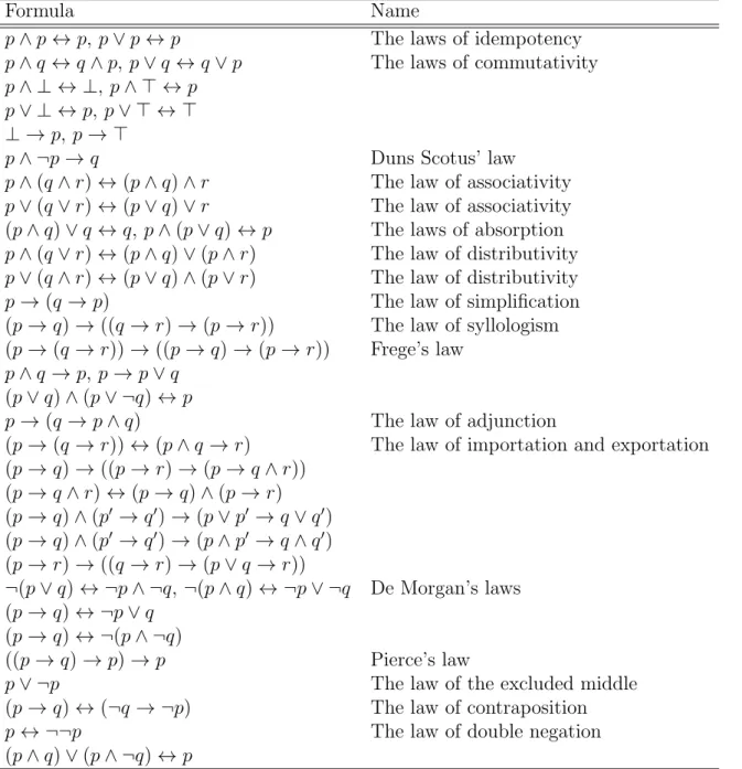
There are lots of well-known valid formulas in classical logic, listed in table 3.1, which we often use in this section. Some formulas in this table overlap with the axioms. Note that the formulas in this table are valid classically: some formulas are not valid in intuitionistic or intermidiate logics. In modal logics handled in this thesis, however, all of the formulas listed here are valid since these logics are based on classical logic.

Before proving the soundness and completeness theorems, let us define some important notions and prepare some lemmas.

Definition 3.1.1 (Derivation). We say that a sequence φ1, . . . , φn of formulas is a

derivation of formula φ if • φn = φ

• for every 1 ≤ i ≤ n, φi satisfies one of the following; – φi is an axiom;

– ∃j, j′ < i[φj ≡ φj′ → φi]; – ∃j < i[φi ≡ □φj].

We denote by ⊢K φ if a formula φ is derivable in K. Lemma 3.1.2. ⊢K φ→ ψ ⇒ ⊢K □φ → □ψ Proof. (1) φ→ ψ (given) (2) □(φ → ψ) (RN) (3) □(φ → ψ) → (□φ → □ψ) (A11) (4) □φ → □ψ ((2), (3), MP) Lemma 3.1.3. ⊢K □(φ ∧ ψ) ↔ □φ ∧ □ψ Proof. (1) φ∧ ψ → φ (A3)

(28)

Table 3.1: A list of classically valid formulas

Formula Name

p∧ p ↔ p, p ∨ p ↔ p The laws of idempotency

p∧ q ↔ q ∧ p, p ∨ q ↔ q ∨ p The laws of commutativity

p∧ ⊥ ↔ ⊥, p ∧ ⊤ ↔ p p∨ ⊥ ↔ p, p ∨ ⊤ ↔ ⊤ ⊥ → p, p → ⊤

p∧ ¬p → q Duns Scotus’ law

p∧ (q ∧ r) ↔ (p ∧ q) ∧ r The law of associativity

p∨ (q ∨ r) ↔ (p ∨ q) ∨ r The law of associativity (p∧ q) ∨ q ↔ q, p ∧ (p ∨ q) ↔ p The laws of absorption

p∧ (q ∨ r) ↔ (p ∧ q) ∨ (p ∧ r) The law of distributivity

p∨ (q ∧ r) ↔ (p ∨ q) ∧ (p ∨ r) The law of distributivity

p→ (q → p) The law of simplification (p→ q) → ((q → r) → (p → r)) The law of syllologism (p→ (q → r)) → ((p → q) → (p → r)) Frege’s law

p∧ q → p, p → p ∨ q

(p∨ q) ∧ (p ∨ ¬q) ↔ p

p→ (q → p ∧ q) The law of adjunction

(p→ (q → r)) ↔ (p ∧ q → r) The law of importation and exportation (p→ q) → ((p → r) → (p → q ∧ r)) (p→ q ∧ r) ↔ (p → q) ∧ (p → r) (p→ q) ∧ (p′ → q′)→ (p ∨ p′ → q ∨ q′) (p→ q) ∧ (p′ → q′)→ (p ∧ p′ → q ∧ q′) (p→ r) → ((q → r) → (p ∨ q → r)) ¬(p ∨ q) ↔ ¬p ∧ ¬q, ¬(p ∧ q) ↔ ¬p ∨ ¬q De Morgan’s laws (p→ q) ↔ ¬p ∨ q (p→ q) ↔ ¬(p ∧ ¬q) ((p → q) → p) → p Pierce’s law

p∨ ¬p The law of the excluded middle

(p→ q) ↔ (¬q → ¬p) The law of contraposition

p↔ ¬¬p The law of double negation (p∧ q) ∨ (p ∧ ¬q) ↔ p

(29)

(2) □(φ ∧ ψ) → □φ ((1), lemma 3.1.2) (3) φ∧ ψ → ψ (A4) (4) □(φ ∧ ψ) → □ψ ((3), lemma 3.1.2) (5) □(φ ∧ ψ) → □φ ∧ □ψ ((2), (4)) (6) φ→ (ψ → φ ∧ ψ) (A5) (7) □φ → □(ψ → φ ∧ ψ) ((6), lemma 3.1.2) (8) □(ψ → φ ∧ ψ) → (□ψ → □(φ ∧ ψ)) (A11)

(9) □φ → (□ψ → □(φ ∧ ψ)) ((7), (8), The law of syllogism)

(10) □φ ∧ □ψ → □(φ ∧ ψ) ((9), The law of importation and exportation) (11) □(φ ∧ ψ) ↔ □φ ∧ □ψ ((5), (10))

The deduction theorem, which is well-known theorem in the field of mathematical logic, should not hold for K if we want K to be sound with respect to the Kripke semantics as it was formulated for classical logic and intuitionistic logic. So, we have to formulate for modal logic. Before formulation, we need to expand a derivation in K, which could deal with assumptions, and define dependency of a formula.

Definition 3.1.4 (Derivation from a set of assumptions). Let Γ be a set of formulas. A

sequence φ1, . . . , φn of formulas is called a derivation of φ from the set of assumptions Γ

if:

• φn = φ;

• for every 1 ≤ i ≤ n, φi satisfies one of the following: – φi is an axiom;

– φi ∈ Γ;

– ∃j, j′ < i[φj ≡ φj′ → φi]; – ∃j < i[φi ≡ □φj].

We denote by Γ⊢K φ if a formula φ is derivable from a set Γ of assumptions in K. Definition 3.1.5 (Dependency). Let φ1, . . . , φn be a derivation from assumptions. Say

that a formula φk depends on a formula φi in this derivation if one of the following holds:

• k = i;

• ∃j, j′ _{< k.[φ}

(30)

• ∃j < k.[φk≡ □φj and (φj depends on φi)].

Theorem 3.1.6 (Deduction theorem for K). Suppose that Γ, ψ ⊢K φ and there exists a

derivation of φ from the assumptions Γ∪{ψ} in which RN is applied to formulas depending on ψ m≥ 0 times. Then

Γ⊢K □0ψ∧ . . . ∧ □mψ → φ

Proof. Let φ1, . . . , φn be a derivation of φ = φn from Γ∪ {ψ}, in which RN is applied to

formulas depending on ψ m times. We show by induction on 1≤ i ≤ n that Γ⊢K □0ψ∧ . . . ∧ □lψ → φi, (∗)

where l is the number of applications of RN to formulas depend on ψ in the derivation Γ1 ⊢ φ1, . . . , Γi ⊢ φi.

• φi is an axiom

Then, the sequence (1) φi (axiom)

(2) φi → (ψ → φi) (A1)

(3) ψ → φi ((1), (2), MP)

(4) ψ∧ (□1ψ∧ . . . ∧ □lψ)→ ψ (A3)

(5) ψ∧ (□1ψ∧ . . . ∧ □lψ)→ φi ((3), (4), The law of syllogism)

is a derivation of (∗).

• φi is a formula in Γi

Then, the sequence

(1) φi (∵ φi ∈ Γ)

(2) φi → (ψ → φi) (A1)

(3) ψ → φi ((1), (2), MP)

(4) ψ∧ (□1ψ∧ . . . ∧ □lψ)→ ψ (A3)

(31)

Then, the sequence

(1) φi → φi∨ φi (A6)

(2) φi∨ φi → φi (The law of idempotency)

(3) ψ → φi ((1), (2), MP, φi ≡ ψ)

(4) ψ∧ (□1ψ∧ . . . ∧ □lψ)→ ψ (A3)

• φi is obtained from φk ≡ φj → φi and φj by MP

Suppose that RN is applied to formulas depending on ψ in φi, . . . , φk and

φi, . . . , φj l1 and l2 times, respectively. Then, by the induction hypothesis, we

have

Γ⊢K □0ψ∧ . . . ∧ □l1ψ → (φj → φi),

Γ⊢K □0ψ∧ . . . ∧ □l2ψ → φj,

and so, we obtain

Γ⊢K □0ψ∧ . . . ∧ □lψ → (φj → φi), Γ⊢K □0ψ∧ . . . ∧ □lψ → φj, since (1) □0ψ∧ . . . ∧ □l1_ψ → (φ j → φi) (given) (2) (□0ψ∧ . . . ∧ □l1_ψ)∧ (□l1+1_ψ∧ . . . ∧ □l_ψ)→ (□0_ψ∧ . . . ∧ □l1_ψ) _{(A3, l} 1 ≤ l) (3) □0ψ∧ . . . ∧ □lψ → (φj → φi) ((1), (2), MP) (4) □0ψ∧ . . . ∧ □l2_ψ → φ j (given) (5) (□0ψ∧ . . . ∧ □l2_ψ)∧ (□l2+1_ψ∧ . . . ∧ □l_ψ)→ (□0_ψ∧ . . . ∧ □l2_ψ) _{(A3, l} 2 ≤ l) (6) □0ψ∧ . . . ∧ □lψ → φj ((4), (5), MP).

Let us denote □0ψ ∧ . . . ∧ □lψ by ∧₁_≤i≤l□iψ. Then we get the following

derivation, which derives (∗).

(7) ( ∧ 1≤i≤l □i ψ → (φj → φi))→ (( ∧ 1≤i≤l □i ψ → φj)→ ( ∧ 1≤i≤l □i ψ → φi)) (A2) (8) ( ∧ 1≤i≤l □i_ψ _{→ φ} j)→ ( ∧ 1≤i≤l □i_ψ _{→ φ} i) ((3), (7), MP) (9) ∧ 1≤i≤l □i_ψ _{→ φ} i ((6), (8), MP).

(32)

• φi is obtained from φj by RN

(i) φj does not depend on ψ

Then, the sequence (1) □φj (given)

(2) □φj → (ψ → □φj) (A1)

(3) ψ → □φj ((1), (2), MP)

(4) ψ∧ (□1ψ∧ . . . ∧ □lψ)→ ψ (A3)

(5) ψ∧ (□1ψ∧ . . . ∧ □lψ)→ □φj ((3), (4), The law of syllogism)

(ii) φj depends on ψ

Suppose that RN is applied l1 < l times to formulas depending on ψ in

φ1, . . . , φj. By the induction hypothesis, we have

Γ⊢K □0ψ∧ . . . ∧ □l1ψ → φj and so, (1) □0ψ∧ . . . ∧ □l1_ψ → φ j (2) □1ψ∧ . . . ∧ □l1+1ψ → □φj ((1), lemma 3.1.2) (3) □0ψ∧ (□1ψ∧ . . . ∧ □l1+1ψ)→ □1ψ∧ . . . ∧ □l1+1ψ (A4) (4) □0ψ∧ . . . ∧ □l1+1ψ → □φj ((2), (3), The law of syllogism).

We get (∗) by repeating (2)-(4).

Corollary 3.1.7. Suppose that Γ, ψ ⊢K φ and there exists a derivation of φ from the

assumptions Γ∪ {ψ} in which RN is not applied to formulas depending on ψ. Then

Γ⊢K ψ → φ.

In the sequel, we will distinguish a derivation into two categories:

• a derivation in which RN is applied exceptionally to formulas that depend only on

an axioms (derivability will be denoted by ⊢);

• a derivation without this restriction (derivability will be denoted by ⊢∗_).

(33)

3.2 Soundness and Completeness

Theorem 3.2.1. ⊢K φ iﬀ F|= φ for all frames F

Proof. (⇒) Let φ1, . . . , φn be a derivation of a formula φ = φn. Suppose that ⊢K φ. Fix

any frame F. We show F|= φ by induction on the length of derivation.

(A1) φi ≡ ψ → (χ → ψ)

Fix any point x ∈ F and valuation V on F. Suppose that (F, V, x) |= ψ. Now it suﬃces to show

(F, V, x)|= χ → ψ

⇔(F, V, x) |= χ implies (F, V, x) |= ψ,

which is obvious.

(A2) φi ≡ (ψ → (χ → σ)) → ((ψ → χ) → (ψ → σ))

Fix any point x∈ F and valuation V on F. Suppose that

(F, V, x)|= ψ → (χ → σ), (3.1)

(F, V, x)|= ψ → χ, (3.2)

(F, V, x)|= ψ. (3.3)

Now it suﬃces to show (F, V, x)|= σ. By (2) and (3), we have (F, V, x) |= χ. We also have (F, V, x)|= χ → σ by (1) and (3). Hence we have (F, V, x) |= σ.

(A3) φi ≡ ψ ∧ χ → ψ

Fix any point x∈ F and valuation V on F. Suppose that (F, V, x)|= ψ ∧ χ

⇔(F, V, x) |= ψ and (F, V, x) |= χ

Now it suﬃces to show (F, V, x)|= ψ, which is obvious.

(A4) φi ≡ ψ ∧ χ → χ

Fix any point x∈ F and valuation V on F. Suppose that (F, V, x)|= ψ ∧ χ

⇔(F, V, x) |= ψ and (F, V, x) |= χ

Now it suﬃces to show (F, V, x)|= χ, which is obvious.

(A5) φi ≡ ψ → (χ → ψ ∧ χ)

Fix any point x ∈ F and valuation V on F. Suppose that (F, V, x) |= ψ and (F, V, x)|= χ. Now it suﬃces to show

(F, V, x) |= ψ ∧ χ

⇔(F, V, x) |= ψ and (F, V, x) |= χ,

(34)

(A6) φi ≡ ψ → ψ ∨ χ

Fix any point x ∈ F and valuation V on F. Suppose that (F, V, x) |= ψ. Now it suﬃces to show

(F, V, x) |= ψ ∨ χ

⇔(F, V, x) |= ψ or (F, V, x) |= χ,

which is obvious.

(A7) φi ≡ χ → ψ ∨ χ

Fix any point x ∈ F and valuation V on F. Suppose that (F, V, x) |= χ. Now it suﬃces to show

(F, V, x) |= ψ ∨ χ

⇔(F, V, x) |= ψ or (F, V, x) |= χ,

which is obvious.

(A8) φi ≡ (ψ → σ) → ((χ → σ) → (ψ ∨ χ → σ))

(F, V, x)|= ψ → σ, (3.4)

(F, V, x)|= χ → σ, (3.5)

(A9) φi ≡ ⊥ → ψ

Fix any point x∈ F and valuation V on F. Then it is obvious since (F, V, x) ⊭ ⊥.

(A10) φi ≡ ψ ∨ (ψ → ⊥)

Fix any point x∈ F and valuation V on F. Our goal is to show (F, V, x)|= ψ ∨ (ψ → ⊥)

⇔(F, V, x) |= ψ or (F, V, x) |= ψ → ⊥.

There are two cases: (F, V, x)|= ψ or (F, V, x) ⊭ ψ. Both cases are trivial.

(A11) φi ≡ □(ψ → χ) → (□ψ → □χ)

(F, V, x)|= □(ψ → χ) ⇔ ∀y ∈ F[xRy ⇒ (F, V, y) |= ψ → χ], (3.7)

(F, V, x)|= □ψ ⇔ ∀y ∈ F[xRy ⇒ (F, V, y) |= ψ]. (3.8)

Now it suﬃces to show

(F, V, x)|= □χ

⇔∀y ∈ F[xRy ⇒ (F, V, y) |= χ].

Fix any y ∈ F such that xRy. By (7) and (8), we have (F, V, y) |= ψ → χ and (F, V, y)|= ψ and so (F, V, y) |= χ holds. Hence (F, V, x) |= □χ.

(35)

φi is obtained from φk ≡ φj → φi and φj by MP

By the induction hypothesis, we have F |= φj → φi and F |= φj and so obviously

F|= φi holds.

φi ≡ □φj is obtained from φj by RN

Fix any point x∈ F and valuation V on F. Our goal is to show that (F, V, x)|= □φj

⇔∀y ∈ F[xRy ⇒ (F, V, y) |= φj].

Fix any y ∈ F such that xRy. The induction hypothesis yields F |= φj and so

(F, V, y)|= φj holds. Hence (F, V, x)|= □φj.

(⇐) First we show

⊬K φ⇒ (There is a Hintikka system h for the tableau (∅, {φ})).

Then, by corollary 2.5.5, we have h ⊭ φ. Before proving this side, we need to define two terms: consistent and maximal.

Definition 3.2.2 (Consistent tableau). A tableau t = (Γ, ∆) is consistent in K if ∀∆′ ⊆

∆[Γ⊬K

∨

φi∈∆′φi].

Definition 3.2.3 (Maximal tableau). A tableau t = (Γ, ∆) is maximal (relative to φ) if

Γ∪ ∆ = Subφ.

Now suppose that ⊬K φ. Let φ1, . . . , φn be a list of all formulas in Subφ. Define a

sequence of tableaux t0 = (Γ0, ∆0), . . . , tn = (Γn, ∆n) by taking

t0 = (∅, {φ}),

ti+1=

{

(Γi, ∆i∪ {φi+1}) ((Γi, ∆i∪ {φi+1}) is consistent)

(Γi∪ {φi+1}, ∆i) (otherwise).

Note that Γn∪ ∆n = Subφ. Let us show that ti is consistent for 0≤ i ≤ n by induction

on i.

(i = 0)

Obvious by the assumption.

(i = k + 1)

(tk+1 = (Γk, ∆k∪ {φk+1}))

Trivial.

(tk+1 = (Γk∪ {φk+1}, ∆k))

Assume for contradiction that (Γk∪ {φk+1}, ∆k) is not consistent. Then there

is a subset ∆′ ={ψ1, . . . , ψm} of ∆k such that

(36)

At the same time, there is a subset ∆′′={χ1, . . . , χn} of ∆k such that

Γk ⊢K χ1∨ · · · ∨ χn∨ φk+1,

since (Γk, ∆k ∪ {φk+1}) is not consistent. Therefore, there is a subset ∆ =

{σ1, . . . , σl} of ∆k such that ∆′, ∆′′ ⊆ ∆ and

Γk, φk+1 ⊢K σ1 ∨ · · · ∨ σl,

Γk ⊢K σ1∨ · · · ∨ σl∨ φk+1.

By corollary 3.1.7, we have Γk ⊢K φk+1 → σ1 ∨ · · · ∨ σl. However, we could

obtain Γk ⊢K σ1 ∨ · · · ∨ σl, which is contrary to the consistency of tk, by the

following derivation: (1) ∨ 1≤j≤l σj∨ φk+1 (given) (2) φk+1 → ∨ 1≤j≤l σj (given) (3) (φk+1 → ∨ 1≤j≤l σj)→ (( ∨ 1≤j≤l σj → ∨ 1≤j≤l σj)→ ( ∨ 1≤j≤l σj∨ φk+1 → ∨ 1≤j≤l σj)) (A8) (4) ( ∨ 1≤j≤l σj → ∨ 1≤j≤l σj)→ ( ∨ 1≤j≤l σj∨ φk+1 → ∨ 1≤j≤l σj) ((2), (3), MP) (5) ∨ 1≤j≤l σj → ∨ 1≤j≤l σj ∨ ∨ 1≤j≤l σj (A6) (6) ∨ 1≤j≤l σj∨ ∨ 1≤j≤l σj → ∨ 1≤j≤l

σj (The law of idempotency)

(7) ∨

1≤j≤l

σj →

∨

1≤j≤l

σj ((5), (6), The law of syllologism)

(8) ∨ 1≤j≤l σj∨ φk+1 → ∨ 1≤j≤l σj ((4), (7), MP) (9) ∨ 1≤j≤l σj ((1), (8), MP)

Now we show that the tableau tn is disjoint and saturated. (disjoint)

Assume for contradiction that tn is not disjoint. Then, there is a formula

ψ such that ψ ∈ Γn and ψ ∈ ∆n. Let Γ′n ≡ Γn∖ {ψ}. It is obvious that

Γn ∪ {ψ} ⊢K ψ. However, since tn is consistent and ψ ∈ ∆n, we have

Γ′_n∪ {ψ} ⊬K ψ. (saturated)

(37)

(S1)

Suppose that ψ∧ χ ∈ Γn and, for contradiction, ψ ∈ ∆n. Then, the

sequence

(1) ψ∧ χ (∵ ψ ∧ χ ∈ Γn)

(2) ψ∧ χ → ψ (A3)

(3) ψ ((1), (2), MP)

is a derivation of Γn ⊢K ψ. However, since tnis consistent and ψ ∈ ∆n,

Γn ⊬K ψ. Hence ψ /∈ ∆n and so ψ∈ Γn as tn is disjoint.

(S2)

Suppose that ψ∧ χ ∈ ∆n and, for contradiction, ψ, χ∈ Γn. Then, the

sequence (1) ψ (∵ ψ ∈ Γn) (2) χ (∵ χ ∈ Γn) (3) ψ → (χ → ψ ∧ χ) (A5) (4) χ→ ψ ∧ χ ((1), (3), MP) (5) ψ∧ χ ((2), (4), MP)

is a derivation of Γn ⊢K ψ ∧ χ. However, since tn is consistent and

ψ∧ χ ∈ ∆n, Γn ⊬K ψ∧ χ. Hence ψ, χ /∈ Γn and so ψ ∈ ∆n or χ∈ ∆n

as tn is disjoint.

(S3)

Suppose that ψ ∨ χ ∈ Γn and, for contradiction, ψ, χ ∈ ∆n. Then,

since tn is consistent, Γn ⊬K ψ∨ χ holds. However, it is obvious that

Γn ⊢K ψ∨ χ since ψ ∨ χ ∈ Γn. Hence ψ, χ /∈ ∆n and so ψ ∈ Γn or

χ∈ Γn as tn is disjoint.

(S4)

Suppose that ψ∨ χ ∈ ∆n and, for contradiction, ψ ∈ Γn. Then, the

sequence

(1) ψ (∵ ψ ∈ Γn)

(2) ψ → ψ ∨ χ (A6)

(3) ψ∨ χ ((1), (2), MP)

is a derivation of Γn ⊢K ψ ∨ χ. However, since tn is consistent and

ψ ∨ χ ∈ ∆n, Γn ⊬K ψ ∨ χ. Hence ψ /∈ Γn and so ψ ∈ ∆n as tn is

disjoint. (S5)

JAIST Repository: Investigation of Modal Logics with Application to Agent Communication [課題研究報告書]