A Statistical Model of Vortex Filaments (Coherent Vortical Structures : Their Roles in Turbulence Dynamics)

A

Statistical

Model of Vortex

Filaments

Zensho YOSHIDA

University of Tokyo, Graduate School of Frontier Sciences

吉田善章

東京大学大学院新領域創成科学研究科

1 Introduction

The Beltrami condition describes the alignment of the vector field and its own vorticity.

In many different $\mathrm{c}o$nvective nonlinear systems, such as fluids and plasmas, the Beltrami

condition plays an important role in characterizing self-organized structures.

A plasmaflow inducesmixingof magneticflux. The length scalecascades toward a small

scale, resultingin amplification of the magneticfield. If theenhanced Lorentz force becomes

to dominate the dynamics, its back-reaction must be taken into account. The Beltrami

condition, which reads as the magnetic force-free condition, must apply to slow motion

of a _{strongly magnetized plasma, i.e., the magnetic field} $B$ must satisfy $\nabla\cross B=\lambda B$

.

This relation characterizes _{the local structure of stable vorteses. In this paper, we derive}

a Boltzmann distribution of the size of _{the filaments that maximizes the entropy for an}

ensemble defined by the total current. An interesting assertion is that the time series

produced by arandom-motionmodel ofsuchfilaments generates apower-law spectrawhich

agrees well with experimantal observation [1].

2 Intermittency

Intermittency is one of the common issues in various complex systems. The underlying

mechanismmay be eitherlow-dimensional chaoticdynamics or high-dimensional statistical

dynamics. A typical example of the latter category is the fluid turbulence [2]. When a

turbulent flow has filamentary structures of vortex tubes, local measurements ofthe flow,

or other related physical quantities, detect _{intermittent fluctuations. Three-dimensional}

shear flows stretch vortex tubes and produce thinner tubes carrying stronger vorticities

(Kelvin’s circulation law), and hence, the vorticity ($\omega=\nabla\cross v;v$ is the flow) tends to

concentrate into filamentary tubes.

Inplasmas, the induction effect and_{the corresponding Lorentz back reaction bring about}

coupling between the flow$v$ and the magnetic field $B$,resulting in a considerable

complica-tion of the dynamics. The stretching effect applies also to the magnetic flux, and $B$ tends

quantities exhibit intermittent behavior and filamentary structures. In the solar

photo-sphere, magnetic field strengths vary in the range of $0$ to 0.2 T. The characteristic length

scale of the magnetic field distribution is of the orderof $100\mathrm{k}\mathrm{m}[3]$

.

Satellitemeasurements

of the magnetotail of the earth detect intermittent fluctuations in ion bulk velocities and

magnetic fields [4].

We consider the filamentation of the electric current $j=\nabla\cross B/\mu_{0}(\mu_{0}$; vacuum

per-meability), which is the vorticity of the magnetic field in a plasma. The reduction of the

length scale of the magnetic field has been discussed by many authors in its relation to

the turbulent cascade process and self-organizations $[5, 6]$

.

The induction effect due to

turbulent plasma flow brings about stretching of flux tubes and generates locally-stable

flux filaments [6]. Such filamentarystructures ofmagnetic fields resemble those of vortices

created in three-dimensional turbulent flows [7]. While eachfilamentary flux tube, such as

aBeltrami field [6], canbe locally stable, theirmovement and mutual interactions are very

complicated [8], and hence, they invoke a statistical mechanical treatment.

Some experimental observations also giveus a motivation to develop amodelof strongly

irregular current in a turbulent plasma. Measurements oflocal currents in turbulent

plas-mas show intermittent fluctuations. In a reversed-field-pinch plasma, internal currents

were measured by inserting a small electrostatic energy analyzer [9]. The data exhibit

strong fluctuations, suggesting that the current density has strongly inhomogeneous

distri-butions [10]. We observe similar behavior on REPUTE-I [11] (Fig. 1).

$\overline{\mathrm{b}\sim\triangleleft}$

$\underline{\Xi}$

$.\wedge-\vee\neg$

UIIE$\mathrm{L}^{\mathrm{l}11\mathrm{O}}\mathrm{J}$

T. SuzukiandZ.Yoshida,Fig.1

Figure 1: The waveform of the local current density (toroidal component) measured inside

the plasma. Thedistance ofthe detectorfrom the center is 75% ofthe radius of the plasma

column. The detector is directed parallel to the local magnetic field during the flat top

phase of the discharge.

while the system is in amacroscopic quasi-steady state. Such a system is insuperablefrom

the viewpoint of conventional theories such as the diffusion model of the current density

or the _{magnetohydrodynamic relaxation model} [12].

3 Statistical Model of Filaments

We apply a statistical mechanical method to characterize the spectral structure of the

current-density fluctuations. The principal macroscopic parameter that characterizes the

system is the total current, _{which is a controllable stationary parameter. We note that we}

do not invoke “energy” to characterize the system. We are not discussing the dynamical

process of_{generating filaments or the dynamics of many filaments, and hence, the energy}

arguments do not apply. Because of the resistive dissipation, the energy is not in

equilib-rium. The filamentary structure ofthe current yields an enhanced dissipation. In such a

“dissipative structure”, _{fluctuations creating filaments yield large dissipation, so that the}

principle of the minimum_{energy dissipation is invalidated.}

The total current is the integral (sum) of local currents (filament currents). We study

the most probable statistical distribution of filament currents for a given total current.

Theoretical predictions will be compared with experimental _{observations.}

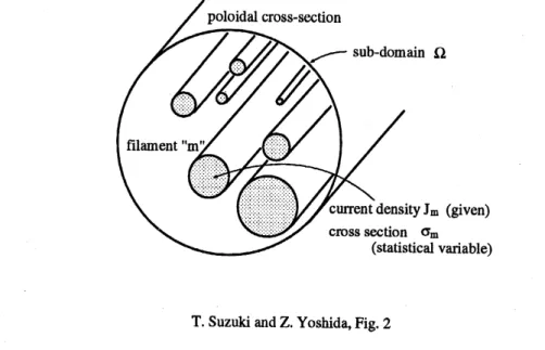
T. SuzukiandZ.Yoshida,Fig.2

Figure 2: A model of current filaments in a plasma column.

Let us consider a system of current filaments. Each filament is denoted by an index $m$

($m=1,$$\cdots,$$N;N$is the total number offilamentsin theensemble). We specify the current

density $J_{m}$ on each filament. The toroidal component is given by

$J_{m}=J_{m}\cdot n$, where $n$

is the unit vector in the toroidal direction. We can invoke the analogy of the standard

statistical mechanics ofparticles, where $J_{m}$ parallels the energy level of the eigenstate

$m$

.

The cross section $\sigma_{m}$ of the filament _$m$ is the statisticalvariable of the present

model $(\sigma_{m}$

may be regarded as the number of particles _{allocated to the eigenstate} $m$). Each filament

We consider a sub-domain $\Omega$ of the total cross section ofthe plasma column as to be a

canonical ensemble that contains $N$ filaments. This $N$ may change, as a grand canonical

ensemble; however, it is appropriate to assume that the “chemical potential” is zero. The

total current in $\Omega$ is given by

$($

$I= \sum_{m=1}^{N}I_{m}=\sum m=N1J_{m}\sigma_{m}$

.

(1)

A micro-state is characterized by specifying $\ell\equiv\{\sigma_{1}, \sigma_{2}, \cdots, \sigma_{N}\}$

.

The probability of a

micro-state$\ell$ is denoted by $p(\ell)\equiv p(\sigma_{1}, \sigma_{2}, \cdots , \sigma_{N})$

.

We haveto normalize the probability

by imposing

$P= \sum_{\ell}p(\ell)\equiv 1$, (2)

where the summation is taken over all possible micro-states. The expectation value of the

current is given by

$(I)= \sum_{\ell}p(\ell)I(\ell)$, (3)

where $I(l)$ is the current of the micro-state$\ell$;

$I( \ell)\equiv I(\sigma 1, \sigma 2, \cdots, \sigma_{N})=\sum_{m}J_{m}\sigma m$

.

(4)

We derive the probability distribution by maximizing the Shannon entropy

$S=- \sum_{l}p(l)\ln p(\ell)$

.

(5)

The use of the Shannon entropy is appropriate when we can assume that the whole

sys-tem of filaments are statistically homogeneous (in a more restricted system, we use the

R\’enyi entropy). Apparently, somefilaments are connected through turns around the torus.

However, we neglect the long-range correlations through toroidal turns, assuming that the

current channels are strongly chaotic. For the above-mentioned canonical ensemble, we

maximize

$H=S-\alpha P-\beta\langle I\rangle$, (6)

where $\alpha$ and $\beta$ are Lagrange multipliers. Thereciprocalof$\beta$ represents the “temperature”

of fluctuati$o\mathrm{n}\mathrm{s}$

.

The variation principle $\delta H=0$ yields the canonical distribution

$p(\ell)=\exp(-\alpha-\beta I(\ell))$

.

(7)

The normalization condition (2) determines $\alpha$;

$Z \equiv\exp(\alpha)=\sum_{\ell}\exp(-\beta I(\ell))$

.

(8)

This $Z$ is the partition function of the canonical distribution.

The probability (7) now reads

We assume that the probability for a filament “

$m$” to have a cross-section $\sigma_{m}$ (denoted by

$p_{m}(\sigma_{m}))$ is independent to the all other filaments. Then, $p(\sigma_{1}, \sigma_{2}, \cdots, \sigma_{N})$ can be broken

down into the simple product of$p_{m}(\sigma_{m})(m=1, \cdots, N)$, and we obtain the “Boltzmann

distribution”

$p_{m}( \sigma_{m})=\frac{\exp(-\beta Jm)\sigma_{m}}{Z_{m}}$, (10)

where

$Z_{m}= \sum_{\sigma_{m}}\exp(-\beta J_{m}\sigma m)$

.

(11)

The inverse temperature $\beta$ characterizes the intensity of fluctuations. For a certain

$\sigma$,

we observe

$\frac{p_{m}(\sigma)}{\Sigma_{k}p_{k}(\sigma)}$ $=$ $\frac{Z_{m}^{-1}\exp(-\beta J_{m}\sigma)}{\Sigma_{k}Z_{k}^{-1}\exp(-\beta J_{k}\sigma)}$

$=$ _{$\frac{1}{1+\Sigma_{k}\neq m(Zm/zk)\exp(-\beta\sigma(Jk-J_{m}))}$}

$\equiv$ $\frac{1}{1+A_{m}}$

.

(12)

In the limit of zero temperature $(\betaarrow\infty),$ _{$A_{m}=0$} for the filament _$m$ that satisfies

$J_{m}= \min_{k}(J_{k})$, and $A_{m}=$ oo for other filaments. This implies that the whole current

condensates on the “grand state”, that is the filament which has the minimum current

density $\sqrt\min$

.

This $J_{\min}$ must be the average current density over the cross section $\Omega$, and

then, $\sigma$ is the total area of$\Omega$

.

Therefore, the current distributes homogeneously on $\Omega$

.

By calculating the total ohmic dissipation produced by a local resistivity $\eta$, we easily

find that the effectiveresistivity for the mean current is given by

$\eta^{*}=\eta\frac{(J^{2}\rangle}{\{J)^{2}}$

.

(13)

In the limit of $\betaarrow\infty,$ $\eta^{*}=\eta$, while a finite $\beta$ yields an enhancedeffective resistivity.

4 Time Seriese Generated by Ramdom Motion of Filaments

Using the probability distribution (10), we generate the time series of the current density

$j(t)$ that is measured at a fixed position in $\Omega$

.

Note that the

probability of measuring the

filament $m$ differs from $p_{m}(\sigma_{m})$ (the probability ofthe filament _$m$ to have a cross section

$\sigma_{m})$

.

We denote by _{$q_{m}$} the probability ofmeasuring a filament

$m$ at afixed point, which is

proportional to $\sigma_{m}$

.

Here, we assume that the filaments cover $\Omega$, and set

$q_{m}= \frac{\sigma_{m}}{|\Omega|}$, (14)

where $|\Omega|$ is the area of $\Omega$

.

To evaluate the period of a certain filament being measured at the observation point, we

specify the speed $v$, which is perpendicular to the toroidal direction, of the filament. We

assume that $v$ is common for allfilaments. Let

$\rho_{m}$ be the radius of the filament $m$;

The duration of the filament $m$ appearing in the time series is given by

$\Delta t_{m}=\frac{2_{\beta m}}{v}$

.

(16)

When we choose a filament $m$, we have the pulse height $J_{m}$ and the pulse width $\Delta t_{m}$ in

the graph of$j(t)$

.

The probability of choosing the filament $m$ must be proportional to the

“cross section” $\rho_{m}\propto\sigma_{m}^{1/2}$

.

The long-term average of the total duration of the filament $m$

appearing in$j(t)$ is given by $\rho_{m}\Delta t_{m}\propto\sigma_{m}\propto q_{m}$, which is consistent with (14).

4.0 _{$\beta=1$ –} $\beta=1\sigma----$ $3.0$ $\frac{\wedge}{\mathrm{v}}$ $\sim$ 2.0 $.\wedge\vee.\neg$ 1.0

$—–$

$-$ $-$ 0.0 1.0 2.0 3.0 4.0 time [msl

T.Suzuki and Z.Yoshida,Fig. 3

Figure 3: Time series$j(t)$ produced by the statistical $\mathrm{m}o$del ($\beta=1$ and $\beta=10^{5}$).

Controllable parameters in the present statistical model are the velocity $v$, the number

of filaments $N$, the “energy level” $\{J_{1}, J_{2}, \cdots, J_{N}\}$, and the inverse temperature $\beta$

.

By

choosing an appropriate set of parameters, we can reproduce the spectral structure of the

experimentally observedfluctuations of the current density. In Fig. 3, we show an example

of the time series $j(t)$ generated by the model with assuming $v=2\mathrm{k}\mathrm{m}/\mathrm{s},$ $N=100$ and

$\beta=1$

.

We also show the non-fluctuating time series given by $\beta=10^{5}$

.

Here, $\{J_{m}\}$

distributes uniformly, with respect to $m$, over the interval $(0, J_{\max}]$

.

We normalize $J_{\max}$

by imposing that (J) $= \sum_{m}J_{m}q_{m}$ gives the mean current density. The typical value of

$\sigma_{m}$ is about 1/200 of the cross section $|\Omega|$

.

To compare with the experiment (Fig. 1),

we take the radius of $|\Omega|$ to be 0.$22\mathrm{m}$

.

The average radius of a filament (defined by

$\rho_{\mathrm{c}}=\Sigma_{m}\rho_{m}J_{m}/\Sigma_{m}J_{m})$ is 1.67 $\mathrm{x}10^{-2}\mathrm{m}$

.

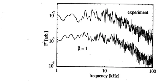
Figure 4 shows the frequency spectrum of$j(t)$ in Fig. 3, in comparison with the

experi-mental spectrumcorresponding to Fig. 1. We observe that the theoretical spectrum agrees

well with the experimental one. The spectrum of$j(t)$ has two distinct frequency ranges;

frequency range $(f>f_{c})$, the _{spectrum is the} $1/f$ spectrum. In the theory, the critical

frequency $f_{\mathrm{c}}$ is given by

$f_{c}= \frac{1}{\pi\Delta i_{c}}=\frac{v}{2\pi\rho_{c}}$, (17)

where $\rho_{\mathrm{c}}$ is the average radius and $\triangle t_{\mathrm{c}}$ is the average duration of a filament;

cf. (16). In

the above example, $\rho_{c}=1.67\cross 10^{-2}\mathrm{m}$ and $v=2\mathrm{k}\mathrm{m}/\mathrm{s}$ yield $f_{c}\simeq 20\mathrm{k}\mathrm{H}\mathrm{z}$

.

T.SuzukiandZ.Yoshida,Fig.4

Figure 4: Power spectrum of$j(t)$ produced by the statistical model _{(Fig. 3), in comparison}

withtheexperimental _{spectrum corresponding to Fig. 1. Weapply different normalizations}

to both spectra to plot them at different vertical positions. A triangle filter (weighted by

3 point for both sides) is applied.

The two different frequency ranges of the spectrum can be explained as follows. In a

long time scale $(|t_{1}-t_{2}|>\triangle t_{c}),$ $j(t_{1})$ and $j(t_{2})$ come from different randomly-selected

filaments. Therefore, we obtain a white spectrum. Agreement of our theoretical result

withthe experimental spectrum_{in this frequency rangejustifies our assumption of random}

movement of filaments.

In the short time _{scale range, the shape of each pulse (height} $=\sqrt m$ and width $=\Delta t_{m}$)

dominates the spectral _{structure. The Fourier transform of a rectangular pulse yields}

$F_{m}(f) \propto|\frac{\sqrt m}{f}\sin(\pi\Delta t_{m}f)|$

.

(18)

Summing up (18) for various pulses “

$m$”, we obtain the $1/f$ spectrum for the frequency

range of $f>f_{c}$

.

Therefore, the $1/f$ spectrum in the high frequency range _{implies that}

the current _{density is approximately uniform in each filament, which justifies the model of}

5 Summary

We have derived a statisticalmodel of filament currents ina plasma, which reproduces the

characteristic structure of thefrequency spectrum ofintermittent current fluctuations. The

theory gives the Boltzmann distribution of the size $\sigma_{m}$ offilaments under the constraint of

thetotal current. An interesting assertionis that the time series produced by the model has

non-Gaussian power-law spectra, although the statistical distribution of $\sigma_{m}$ is Gaussian.

This is because the spectrum of the time series is primarilycharacterized bythe probability

$q_{m}\propto\sigma_{m}$ (see (14)) where$p_{m}(\sigma_{m})\propto\exp(-\beta J_{m}\sigma_{m})$

.

The authors are grateful to the REPUTE experiment group for their discussions. This

work wassupported by Grant-in-Aidfor Scientific Research from the Japanese Ministry of

Education, Science and Culture No. 09308011.

References

[1] T. Suzuki, Intermittent Fluctuations

_of

internal Current in a Turbulent Plasma,

dis-ertation, University ofTokyo (1999).

[2] Y. Couder, S. Douady and O. Cadot, $\tau_{ur}bulence_{J}$ A Tentative Dictionary, edited by

P. Tabeling and O. Cardoso (Plenum, New York, 1995), p.131.

[3] J. O. Stenflo, Sol. Phys. 32, 41 (1973).

[4] V. Angelopoulos et al., J. Geophys. Res. 97, 4027 (1992).

[5] D. Biskamp and H. Walter, Phys. Fluids B1, 1964 (1989); Phys. Fluids B2, 1787

(1990).

[6] Z. Yoshida, Phys. Rev. Lett. 77, 2722 (1996).

[7] E. D. Siggia, J. Fluid Mech. 107, 375 (1981).

[8] The dynamics of a system ofcurrent filaments was studied by Y. Yatsuyanagi, T.

Ha-tori and T. Kato, J. Phys. Soc. Jpn. 65, 745 (1996); see also D. W. Moore and

P. G. Saffman, Philos. Trans. R. Soc. Lond. Ser. A 272, 403 (1972); R. Kinney,

T. Tajima, J. C. McWilliams and N. Petviashvili, Phys. Plasmas 1, 260 (1994).

[9] J. C. Ingraham et al., Phys. Fluids B2,143 (1990).

[10] A plasma with imperfect magnetic surfaces must have a microscopically filamented

current structure; see J. B. Taylor, Phys. Fluids B5, 4378 (1993).

[11] Z. Yoshida et al., J. Plasma Phys. 59, 103 (1998).