Quantifying Sentiment for the Japanese Economy and Stock Price Prediction

全文

(1)IPSJ SIG Technical Report. Vol.2014-MPS-99 No.13 2014/7/21. Quantifying Sentiment for the Japanese Economy and Stock Price Prediction HIROSHI ISHIJIMA†1 TAKURO KAZUMI†2 AKIRA MAEDA†3 The purpose of this paper is to re-examine the analysis of Ishijima et al. [2], providing a more comprehensive analysis on the sentiment of the Japanese economy that appears on the Nikkei articles. We extend their analysis in two dimensions: One is to expand data coverage, and the other is to create variations of the original sentiment index. Granger causality test results indicate the usefulness of our sentiment indexes. Keywords: Big data, Text mining, Nikkei, Sentiment, Stock market. 1. Introduction. ,. Sentiment analysis is gaining increasing interest in both academia and businesses. As the sentiment invisibly reflects the atmosphere of economic activities and the psychology of economic agents, analyzing the sentiment helps us understand the economy and security markets in a more sophisticated way. With such a conception, Ishijima et al. [2] analyzed the sentiment towards the Japanese economy that might appear in daily news articles. In fact, they created an index that accounts for the frequency of occurrence of words that affirmatively or negatively describe the current economic situation. Articles were taken from the Nikkei, a popular business newspaper in Japan. They then performed statistical analysis to examine correlations between the sentiment index and Tokyo Stock Exchange prices. Interestingly, they concluded that the index significantly predicts stock prices of three days in advance. The purpose of this paper is to re-examine the analysis of Ishijima et al. [2], providing a more comprehensive analysis on the sentiment of the Japanese economy that appears on the Nikkei articles. To this end, we extend their analysis in two dimensions: One is to expand data coverage, and the other is to create variations of the original sentiment index. The rest of this paper is organized as follows. Section 2 elaborates on how to create sentiment indexes. Section 3 builds our models. Section 4 implements an empirical analyzes in the Japanese stock markets. Section 5 concludes the paper.. 2. Creating Sentiment Indexes 2.1 Source: the coverage of pages to pick words Every page in newspapers is comprised of pairs of headlines and articles. The place where the word appears either in headlines or in articles might affect the impact of how much the reader will invoke positive or negative sentiment on that word. In this aspect, we strictly distinguish the words in articles from the words in headlines. We clarify on this by introducing some notations. In the newspapers delivered at day , we have and. ( ). ( ). headlines. articles. Each headline and article are denoted by. †1 Chuo University and Columbia Business School †2 CyberAgent, Inc.. ⓒ2014 Information Processing Society of Japan. ( ). = 1, ⋯ ,. and. ,. and. ( ) ,. and article have. ( ) ,. in headline. and article. 1, ⋯ ,. ( ) ,. ,. and. ( ) ,. = 1, ⋯ ,. ( ). . Each headline. words, respectively. The words ,. are denoted by. = 1, ⋯ ,. ( ) ,. ( ) ,. =. , respectively.. At this point, we introduce the aggregate notation to represent whichever the word that comprises either headlines or articles. This enables us easier to articulate how to quantify the sentiment in the discussion that will follow. The coverage of pages to pick words is limited to either headlines or articles and is denoted by ≔ , . We simply call as the “source.” We then let ∈ to show either headline or article .Then in the newspaper delivered at day 1, ⋯ ,. ( ) ,. ( ) ,. ,. denotes the. that comprises the -th source. =. -th word ,. = 1, ⋯ ,. ( ). .. 2.2 Semantic dictionary The semantic dictionary (Takamura, [3]) is denoted by ≔ , ( ) = 1 ⋯ . That is, the dictionary comprises pairs of word and its semantic score that ranges from -1 to +1. Regarding the semantic score, the closer to -1 (or +1) the score becomes, the more negative (or positive) feeling the word invokes to the Japanese people. 2.3 Semantic index: two methods to quantify the positive or negative feelings We define the indicator function to count if the word that appears in the source matches one of listed words in the dictionary. ( ) , (. )≔. 1. if. ( ) ,. matches. 0 (otherwise). (1). In the aspects of how to score the positive or negative feelings, we introduce two methods to create the sentiment indexes. (1) Real-valued sentiment index = ( ) that is The first way is to exploit the semantic score . We define this first way as the assigned to the listed word †3 The University of Tokyo. 1.

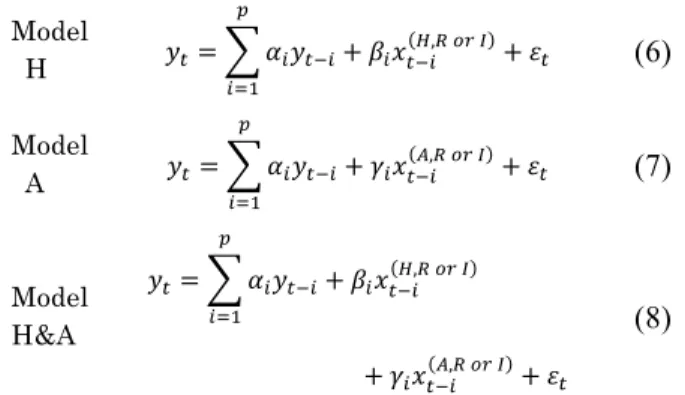
(2) IPSJ SIG Technical Report. Vol.2014-MPS-99 No.13 2014/7/21. “real-valued sentiment index:” ( ). ( , ). ( ) ,. ( ) , (. ≔. )⋅. (2). For the source = that the coverage of pages to pick words is limited to headlines, the real-valued sentiment index is given by. ( , ). =. ( , ). . In the same way, for the source of. (articles), the real-valued sentiment index is given by ( , ). ( , ). Model H. =. +. ( ,. ). +. (6). Model A. =. +. ( ,. ). +. (7). = =. Model H&A. =. ( ,. +. (8) +. .. (2) Integer-valued sentiment index to the nearest The second way is to round the semantic score binary integer that is either -1 or +1. Introducing the integer variable for each of semantics scores: ≤ 1) +1 (if 0 < ≔ (3) −1 (if − 1 ≤ < 0) We then define the second way as “integer-valued sentiment index”: ( ). ( , ). ≔. ( ) ,. ( ) , (. )⋅. (4). Reminding that each of two sentiment indexes has the option in picking the source, – either headlines ( = ) or entire set of articles ( = ) – we thus have four types of sentiment indexes in the analysis. As a summary, we use the following notation to represent these four sentiment indexes (s.i.).. ). ( ,. ). +. Within these VAR(p) model specifications, the Granger causality can be stated if the sentiment indexes ( ( ,#) ) Grangercause (G-cause) stock log-returns ( ), the past sentiment indexes should help predict the stock log-returns, beyond prediction by past stock log-returns alone. Using these three VAR(p) models, we will implement the three Granger causality tests (G-tests). (1) “G-test for Model H” tests whether or not the headline sentiment index G-causes stock log-returns by exploiting = 0 ( = 1 ⋯ ). Equation (6). The null hypothesis is (2) “G-test for Model A” tests whether or not the entire article sentiment index G-causes stock log-returns by exploiting Equation (7). The null hypothesis is = 0 ( = 1 ⋯ ). (3-1) “G-test 1 for Model H&A” tests whether or not the headline sentiment index G-causes stock log-returns by exploiting Equation (8). The null hypothesis is = 0 ( = 1 ⋯ ). (3-2) “G-test 2 for Model H&A” tests whether or not the entire article sentiment index G-causes stock log-returns by exploiting Equation (8). The null hypothesis is = 0 ( = 1 ⋯ ).. ( ,#) ( , ). (integer − valued headline s. i. ) (real − valued headline s. i. ) (5) ≔ ( , ) (integer − valued article s. i. ) ( , ) (real − valued article s. i. ) where denotes one of the sources or and # denotes the scoring method that is either integer-valued “ ” scoring or real-valued “ ” scoring. Along the procedures that we described above, we created 29year daily time-series of four sentiment indexes based on headlines and articles from the Nikkei. We remark that these sentiment indexes are normalized so that they have zero means and unit standard deviations. Due to space limitation, we omitted reporting summary statistics and time-series charts of our sentiment indexes. ( , ). 3. Model To explore whether or not our sentiment indexes are able to predict stock prices, we will exploit the vector auto-regression (VAR) model that is conventional one in the econometrics literature. For each of two cases in terms of the scoring method, we estimated three VAR(p) models which comprise either (1) Model H: headline sentiment index, (2) Model A: entire article sentiment index, (3) Model H&A: both headline and article sentiment indexes, as well as stock log-returns. Namely, each of three models is specified as follows:. ⓒ2014 Information Processing Society of Japan. 4. Empirical Analysis in the Japanese Stock Market While the Nikkei is daily published and delivered with a few noissue days, the Japanese stock market is closed every weekend. To handle such daily data set that is partially missing and hence inconsistent in frequency, we follow the approach of Bollen et al. [1]. That is, we eliminated every Saturday and Sunday from complete data set before implementing analysis. Also, before estimating VAR models Eqs. (6)‒(8), we implemented augmented Dickey–Fuller tests. For each year, we verified that all the time series of stock log-returns, headline and article sentiment indexes do not have unit root with 1% significance. Table 1 and Table 2 show Granger test results with real- and integer-valued sentiment indexes, respectively. For each year, three models of Model H, A and H&A or relevant Eqs. (6), (7) and (8) are estimated and tested. On each model estimation, we searched the lag from 1 to 7 to identify the best (i.e. lowest) in terms of AIC. For each model estimation with the best , the relevant test statistics (“Granger”-labeled columns) and AIC values are reported in Tables. Table 1: Predictability of “real-valued sentiment index” in terms of Granger tests and AICs. Test statistics for Granger causality. 2.

(3) IPSJ SIG Technical Report. Vol.2014-MPS-99 No.13 2014/7/21. are given in the columns titled “Granger.” *, ** and *** mark the test statistics that are 10%, 5% and 1% significant, respectively. Headline Eq. (6) Article Eq. (7) Headline & Article Eq. (8) Year Lag (p) Granger AIC Lag (p) Granger AIC Lag (p) Granger H Granger A 1984 3 1.12 -10.17 6 1.51 -10.10 6 4.99*** 5.20*** 1985 7 1.54 -10.46 6 1.78 -10.65 6 3.60*** 3.67*** 1986 2 1.69 -10.18 6 1.00 -10.44 6 1.91** 1.17 1987 2 0.02 -9.21 6 1.78 -9.77 6 0.71 1.64* 1988 2 1.12 -11.07 6 0.66 -11.38 6 1.88** 1.28 1989 2 2.89* -11.53 5 1.39 -12.01 5 1.98** 1.86** 1990 2 0.14 -8.73 7 1.96* -9.63 5 3.30*** 4.75*** 1991 2 0.40 -9.37 5 0.52 -10.35 5 3.48*** 4.93*** 1992 5 1.29 -8.69 5 0.83 -9.48 5 2.06** 2.69*** 1993 1 1.67 -9.18 5 0.21 -10.03 5 3.17*** 3.69*** 1994 1 0.41 -9.46 5 0.37 -10.27 5 1.77* 5.12*** 1995 5 0.94 -9.19 5 0.37 -9.98 5 3.91*** 4.71*** 1996 5 1.08 -10.05 5 0.53 -11.08 5 1.70* 2.24** 1997 2 0.07 -8.78 5 1.18 -9.72 5 2.31** 2.49*** 1998 5 3.01** -8.80 5 2.22* -9.94 5 1.43 3.23*** 1999 1 0.64 -9.29 5 0.29 -9.99 5 1.60 2.20** 2000 1 4.35** -8.99 5 1.37 -10.04 6 1.77** 3.74*** 2001 2 0.32 -8.59 1 0.36 -9.72 1 2.19 2.31* 2002 2 2.03 -8.90 5 0.94 -10.10 5 0.77 1.42 2003 1 0.12 -8.89 5 0.25 -10.30 1 0.54 2.59* 2004 1 0.16 -9.50 5 1.30 -10.70 1 0.19 2.74* 2005 5 0.18 -10.10 5 0.30 -11.24 1 4.29** 8.65*** 2006 5 0.70 -9.37 5 1.74 -10.53 5 1.07 3.57*** 2007 6 0.42 -9.59 6 0.15 -10.70 5 2.27** 4.40*** 2008 6 0.37 -7.68 5 0.58 -8.59 5 1.92** 4.48*** 2009 6 0.95 -8.87 6 0.83 -9.88 6 1.51 1.62* 2010 5 2.35** -9.24 5 2.26** -10.36 5 1.51 2.72*** 2011 1 0.19 -9.18 5 1.13 -10.00 5 1.07 1.45 2012 2 3.88* -9.71 5 1.13 -10.91 5 1.20 1.04. AIC -11.19 -11.45 -11.60 -11.17 -12.88 -13.70 -11.21 -11.72 -10.79 -11.29 -11.52 -11.48 -12.61 -11.21 -11.28 -11.22 -11.36 -11.17 -11.74 -11.99 -12.26 -12.81 -12.27 -12.32 -10.15 -11.36 -12.02 -11.44 -12.32. Table 2: Predictability of “integer-valued sentiment index” in terms of Granger tests and AICs. Test statistics for Granger causality are given in the columns titled “Granger.” *, ** and *** mark the test statistics that are 10%, 5% and 1% significant, respectively. Headline Eq. (6) Article Eq. (7) Headline & Article Eq. (8) Year Lag (p) Granger AIC Lag (p) Granger AIC Lag (p) Granger H Granger A 1984 1 0.35 -9.76 1 1.06 -10.04 1 2.77* 2.72* 1985 2 3.03** -10.39 3 3.39** -10.72 1 1.16 0.69 1986 1 2.58 -9.62 1 2.21 -9.49 1 3.56** 0.49 1987 1 0.20 -8.40 6 1.29 -8.70 1 0.28 2.11 1988 2 0.60 -10.37 5 1.87* -10.77 1 0.18 0.98 1989 6 1.92* -10.42 1 2.49 -10.86 1 0.12 1.50 1990 2 0.04 -7.65 2 1.01 -8.16 2 1.16 0.89 1991 1 0.37 -8.69 1 1.36 -9.03 2 2.86** 1.76 1992 1 2.07 -8.28 5 1.04 -8.29 1 0.95 0.23 1993 4 3.51*** -8.81 1 0.03 -9.06 1 0.87 0.03 1994 5 1.32 -9.55 1 0.01 -9.59 1 0.14 0.42 1995 1 0.21 -8.86 1 0.11 -9.28 1 0.19 0.52 1996 1 2.12 -9.33 1 0.12 -9.73 1 1.70 0.44 1997 2 1.04 -8.67 2 0.42 -8.82 2 0.53 0.57 1998 2 0.78 -8.49 5 2.05* -8.78 1 1.43 2.12 1999 1 0.10 -9.35 1 0.05 -9.57 1 0.11 7.06*** 2000 1 0.31 -8.41 1 0.65 -9.11 1 0.86 0.67 2001 1 1.43 -8.28 1 0.02 -8.48 1 3.02** 0.59 2002 1 0.10 -8.82 1 0.91 -9.01 1 0.02 1.70 2003 5 2.88* -8.70 4 1.71 -8.63 1 2.73* 2.29 2004 1 0.01 -9.38 1 0.00 -9.69 1 2.96* 0.23 2005 1 0.48 -9.74 5 0.41 -9.67 5 1.13 1.45 2006 1 0.17 -9.24 2 0.13 -9.70 2 0.86 1.02 2007 1 1.28 -9.06 6 2.21** -9.27 1 2.41* 3.40** 2008 1 0.32 -7.62 3 0.41 -7.68 1 1.04 2.16 2009 3 1.73 -8.38 6 1.57 -8.02 1 6.26*** 0.91 2010 3 1.55 -8.89 5 2.18* -9.22 3 2.64** 1.35** 2011 1 0.10 -8.61 4 2.43** -8.95 1 1.34 3.48** 2012 1 0.87 -9.56 3 0.95 -9.86 1 1.95 0.20. AIC -10.19 -10.83 -9.79 -9.08 -11.15 -11.11 -8.28 -9.39 -8.80 -9.34 -10.31 -9.74 -9.91 -9.48 -9.40 -10.39 -9.23 -9.13 -9.78 -9.10 -10.38 -10.13 -10.30 -9.66 -8.31 -8.60 -9.56 -9.21 -10.36. 4.1 Goodness of fit For both real- and integer-valued cases, Model H&A fits best in terms of AICs throughout 29 years. When comparing the realand integer-valued cases, the former performs better in the aspects of AICs. Hence, in the following discussion, we will mainly focus on the results for estimating Model H&A on the basis of real-valued sentiment index.. ⓒ2014 Information Processing Society of Japan. 4.2 Predictability of stock prices From the right most panel in Table 1, Model H&A of Eq. (8) persistently shows the predictability of stock prices on the basis of real-valued sentiment index. More specifically, the article index persistently and significantly Granger-causes the stock logreturns in conjunction with the headline index (“Granger A” column in that right most panel). Also, the headline index Granger-causes the stock log-returns in conjunction with the article index (“Granger H” column in the same panel). On the flipside, Models H and A (Eqs. (6) and (7)) do not seem to provide the persistent Granger causalities. These results imply that it is important for our VAR modeling to incorporate both headline and article sentiment indexes in order to predict stock prices; and that it is insufficient to separately introduce either headline or article sentiment indexes. It should be noted that the Granger causality seems to be weakened during some periods. We will elaborate on each of these. During the period from 1986 to 1988 that was right after the Plaza Accord on 1985, the Japanese market has been a bull market and on the way to its peak. In this period, the headline sentiment index has stronger Granger causality than the article’s except 1987 that has brought Black Monday. In contrast, during the period from 2001 to 2004 that was right after the burst of the Internet bubble, in the year of 2009 that was right after the 2008 financial crisis, and during two years from 2011 to 2012 in which we experienced the Japan quake and had been trying to recover, the Japanese economy suffered from these unusual events. In those periods, the article index has stronger Granger causality than the headline index. 4.3 Significant lagged variables: Table 3 exhibits the year-on-year estimates of Model H&A of Eq. (8) on the basis of real-valued sentiment index. Interestingly enough, we found the seven cyclical patterns in our estimation results. Cycle 1 was significant: For the first 10 years from 1984 to 1993 except 1986 ‒ that correspond to the 11th business cycle defined by Cabinet Office in Japan ‒, two sentiment indexes with shorter lags (1 to 2) and longer lags (5 to 6) served as significant variables. Cycle 2 was not significant: In the next 5 years from 1994 to 1998 that correspond to the 12th business cycle in Japan, we couldn’t find any significant lagged variables on neither headline nor article indexes. Cycle 3 was significant: In the next 2 years from 1999 to 2000 that correspond to the Internet bubble, two sentiment indexes with lag-of-one and middle lags (3 to 4) were significant. Cycle 4 was not significant: During the period from 2001 to 2005 that was after the burst of the Internet bubble and before 2008 financial crisis, we couldn’t find any significant lagged variables in sentiment indexes, again. Cycle 5 was significant: In the 3 years from 2006 to 2008 that brought the financial crisis, two sentiment indexes with lag-ofone and middle lags (3 to 4) were significant. Cycle 6 was not significant: During the period from 2009 to 2010 that was right after the crisis and corresponded to the very first. 3.

(4) ⓒ2014 Information Processing Society of Japan. 6. 5. 1989. 5. 5. 2006. 2007. 5. 5. 2011. 2012. 5. 1. 2005. 2010. 1. 2004. 5. 1. 6. 5. 2002. 2003. 2008. 1. 2001. 2009. 5. 6. 1999. 2000. 5. 5. 1997. 1996. 1998. 5. 5. 1995. 5. 5. 1993. 1992. 1994. 5. 5. 1991. 5. 6. 1988. 1990. 6. 1987. Acknowledgments Authors would like to thank anonymous referees and organizers of MPS 99, a satellite workshop of PDPTA’14 comprising WORLDCOMP’14 for their useful comments. -0.0405 (0.5335) 0.0083 (0.9016) -0.0861 (0.1994) 0.0563 (0.3903) -0.1084 (0.1059) -0.0082 (0.9023) 0.0724 (0.3592). -0.0305 (0.6504). -0.0011 (0.6233) -0.0012 (0.5323) 0.0037 (0.4140) -0.0035 (0.1583) 0.0018 (0.4134) 0.0024 (0.2670) 0.0044** (0.0108). 0.0013 (0.6261). -0.0003 (0.9405) 0.0013 (0.6547) -0.0018 (0.7847) 0.0037 (0.3547) -0.0036 (0.3153) -0.0065** (0.0404) -0.0050* (0.0822). -0.0031 (0.5006). Art -0.0019*** (0.0078) -0.0011** (0.0211) -0.0006 (0.5621) -0.0020 (0.4570) -0.0005 (0.6257) -0.0009 (0.3362) 0.0006 (0.8865) 0.0022 (0.3471) 0.0000 (0.9944) -0.0011 (0.6709) 0.0014 (0.4440) 0.0024 (0.3752) 0.0010 (0.6320) -0.0049 (0.1803) -0.0019 (0.6163) 0.0006 (0.7911) 0.0001 (0.9722). 3) H. Takamura. (2007). Tango Kanjyo Kyokusei Taiou Hyou (Semantic Orientations Dictionary). [Online]. Available URL: http://www.lr.pi.titech.ac.jp/~takamura/pndic_ja.html (accessed 201405-31) Lag 2 Head 0.0016** (0.0388) 0.0004 (0.4617) -0.0007 (0.4963) 0.0017 (0.4245) 0.0002 (0.7766) 0.0000 (0.9675) -0.0015 (0.6301) -0.0008 (0.6464) 0.0031 (0.2131) 0.0015 (0.3863) -0.0004 (0.8045) -0.0010 (0.6096) -0.0013 (0.3886) 0.0029 (0.2330) -0.0021 (0.3691) 0.0004 (0.8187) 0.0002 (0.9071). 0.0177 (0.7887) 0.0983 (0.1393) -0.0992 (0.1390) -0.0607 (0.3503) 0.1085 (0.1002) 0.0198 (0.7677) 0.0973 (0.2150). 0.0164 (0.8081). Ret -0.0894 (0.1960) -0.0962 (0.1235) -0.0633 (0.3353) 0.0669 (0.2936) -0.0188 (0.7659) 0.0405 (0.5321) -0.0098 (0.8872) -0.0459 (0.4889) 0.0349 (0.5957) -0.0616 (0.3659) 0.0439 (0.5054) -0.0258 (0.6978) 0.0482 (0.4774) -0.0044 (0.9477) 0.1273* (0.0528) 0.0308 (0.6447) -0.1037 (0.1193). 0.0023 (0.2890) -0.0016 (0.4023) -0.0002 (0.9729) 0.0003 (0.9058) -0.0024 (0.2624) -0.0009 (0.6670) 0.0000 (0.9874). -0.0005 (0.8399). Lag 3 Head -0.0011 (0.1588) -0.0003 (0.5829) -0.0004 (0.6666) 0.0011 (0.6203) 0.0001 (0.9308) -0.0019** (0.0283) 0.0036 (0.2445) 0.0007 (0.6917) -0.0012 (0.6280) 0.0019 (0.2527) 0.0019 (0.1878) -0.0014 (0.5042) 0.0017 (0.2388) -0.0018 (0.4399) 0.0022 (0.3533) 0.0029* (0.0886) -0.0018 (0.3445). 2) H. Ishijima, T. Kazumi and A. Maeda, “Sentiment Analysis for the Japanese Stock Market,” forthcoming in Global Business and Economics Review, 2014.. Ret 0.0244 (0.7278) -0.0619 (0.3202) -0.0375 (0.5688) -0.1594** (0.0118) -0.0463 (0.4620) 0.0672 (0.3010) -0.2147*** (0.0015) -0.1459** (0.0297) -0.0157 (0.8130) 0.0131 (0.8480) -0.0495 (0.4534) 0.0183 (0.7811) 0.0622 (0.3572) -0.2213*** (0.0010) -0.1297** (0.0487) -0.0499 (0.4547) 0.0333 (0.6175). -0.0070** (0.0383) 0.0002 (0.9358) -0.0012 (0.8610) -0.0006 (0.8721) -0.0010 (0.7855) -0.0020 (0.5191) -0.0036 (0.2138). -0.0023 (0.6146). Art 0.0009 (0.2099) 0.0001 (0.8982) -0.0002 (0.8704) -0.0018 (0.4950) 0.0005 (0.5971) 0.0020** (0.0397) -0.0055 (0.1721) -0.0005 (0.8331) -0.0008 (0.8029) -0.0026 (0.2948) -0.0020 (0.2830) 0.0021 (0.4187) -0.0012 (0.5624) 0.0056 (0.1200) 0.0008 (0.8232) -0.0031 (0.1806) 0.0054* (0.0591). 1) J. Bollen, H. Mao and X. Zeng, “Twitter Mood Predicts the Stock market,” Journal of Computational Science, vol. 2, no. 1, pp. 1–8, 2011.. Art -0.0006 (0.3393) 0.0007 (0.1773) 0.0010 (0.3474) 0.0056** (0.0362) 0.0014 (0.1627) 0.0002 (0.8145) -0.0074* (0.0633) -0.0022 (0.3424) 0.0031 (0.3393) -0.0008 (0.7460) -0.0006 (0.7481) 0.0019 (0.4632) 0.0001 (0.9741) -0.0038 (0.2854) -0.0014 (0.6893) -0.0005 (0.8207) -0.0021 (0.4806) -0.0021 (0.6284) 0.0041 (0.3760) -0.0041 (0.3399) -0.0003 (0.9136) 0.0010 (0.6425) -0.0040 (0.2178) -0.0063** (0.0301) 0.0062 (0.3388) -0.0028 (0.5007) 0.0001 (0.9696) 0.0020 (0.5220) 0.0007 (0.8024). Reference. 1986. Lag 1 Head 0.0014* (0.0699) -0.0005 (0.3683) 0.0000 (0.9741) -0.0030 (0.1543) -0.0021** (0.0153) -0.0013 (0.1137) 0.0025 (0.4152) 0.0030* (0.0861) -0.0009 (0.7116) 0.0014 (0.4069) 0.0001 (0.9593) -0.0020 (0.3160) -0.0019 (0.1905) 0.0016 (0.4889) -0.0029 (0.2056) 0.0009 (0.5987) 0.0042** (0.0292) 0.0003 (0.9087) 0.0008 (0.7687) 0.0021 (0.3246) 0.0005 (0.7365) 0.0000 (0.9943) 0.0029 (0.1551) 0.0045** (0.0152) -0.0014 (0.7583) 0.0021 (0.3970) 0.0021 (0.3300) -0.0006 (0.7770) -0.0026 (0.1195) -0.0581 (0.3783) -0.1323* (0.0503) -0.0079 (0.9062) 0.1019 (0.1190) -0.0404 (0.5402) -0.2052*** (0.0023) -0.0410 (0.5966). -0.0168 (0.8036). Ret 0.2067*** (0.0031) -0.0169 (0.7859) 0.0927 (0.1586) -0.1119* (0.0805) 0.0119 (0.8327) -0.0771 (0.2289) 0.0369 (0.5831) -0.0589 (0.3792) 0.0487 (0.4570) 0.1002 (0.1461) 0.0638 (0.3283) -0.0561 (0.4000) 0.0873 (0.2023) -0.0900 (0.1682) -0.1350** (0.0387) 0.0515 (0.4393) 0.0573 (0.3802). 0.0007 (0.7324) 0.0006 (0.7358) -0.0085* (0.0634) -0.0014 (0.5845) -0.0008 (0.7165) 0.0016 (0.4540) -0.0001 (0.9404). 0.0017 (0.5311). Lag 4 Head -0.0014* (0.0874) -0.0003 (0.5911) 0.0007 (0.5046) 0.0000 (0.9817) 0.0009 (0.2739) 0.0005 (0.5839) -0.0005 (0.8614) -0.0020 (0.2579) -0.0038 (0.1341) -0.0006 (0.7287) -0.0003 (0.8186) -0.0028 (0.1728) -0.0011 (0.4368) -0.0025 (0.2793) 0.0016 (0.4859) -0.0035** (0.0374) 0.0017 (0.3816). -0.0064* (0.0531) -0.0013 (0.6675) 0.0127* (0.0572) 0.0003 (0.9337) 0.0031 (0.3894) -0.0038 (0.2370) 0.0019 (0.5090). -0.0015 (0.7367). Art 0.0002 (0.8205) 0.0003 (0.5659) -0.0010 (0.2996) 0.0015 (0.5756) 0.0003 (0.7567) 0.0004 (0.7003) -0.0029 (0.4681) 0.0003 (0.8941) 0.0018 (0.5856) 0.0007 (0.7906) 0.0001 (0.9611) 0.0030 (0.2785) 0.0022 (0.2901) 0.0042 (0.2509) 0.0021 (0.5625) 0.0035 (0.1227) -0.0023 (0.4371). 0.0759 (0.2483) -0.0476 (0.4796) -0.0594 (0.3710) -0.0966 (0.1414) -0.1221* (0.0683) 0.0046 (0.9466) 0.0206 (0.7885). 0.0303 (0.6518). Ret -0.1650** (0.0205) -0.0118 (0.8489) 0.0019 (0.9771) 0.1661*** (0.0091) -0.0601 (0.2800) -0.0049 (0.9382) -0.1191* (0.0745) 0.0375 (0.5753) 0.0908 (0.1642) -0.0555 (0.4239) -0.0950 (0.1464) -0.0935 (0.1645) -0.0088 (0.8950) 0.0155 (0.8101) 0.0749 (0.2486) 0.0010 (0.9879) -0.0502 (0.4489). We created the 29-year daily time-series of four sentiment indexes that reflect the positive or negative feelings represented in the Nikkei newspaper. The analysis is based on Ishijima et al. [2], but is a sophisticated version of their analysis. We showed the persistent predictability of Japanese stock prices on the basis of two sentiment indexes that quantified the sentiment over headlines and entire articles, respectively.. 6. Ret 0.2275*** (0.0013) 0.0693 (0.2604) 0.2369*** (0.0002) -0.0254 (0.6876) 0.0502 (0.4276) 0.0200 (0.7612) 0.1275* (0.0566) 0.0331 (0.6228) -0.0328 (0.6239) -0.0191 (0.7766) -0.0804 (0.2246) 0.0335 (0.6124) -0.1412** (0.0356) -0.2031*** (0.0024) -0.0045 (0.9458) -0.0912 (0.1750) 0.0275 (0.6840) -0.1038 (0.1080) -0.0126 (0.8517) 0.0302 (0.6399) -0.0131 (0.8392) 0.0512 (0.4308) -0.0786 (0.2349) 0.0284 (0.6737) -0.0749 (0.2650) -0.0271 (0.6853) 0.0336 (0.6145) 0.0058 (0.9317) 0.0214 (0.7861). 5. Conclusions. 1985. Const -0.0011 (0.5962) 0.0004 (0.5817) 0.0012** (0.0302) -0.0017 (0.4925) 0.0005 (0.5698) 0.0022** (0.0230) 0.0021 (0.5849) -0.0006 (0.7449) -0.0044 (0.2150) 0.0001 (0.9665) 0.0004 (0.8255) -0.0018 (0.3189) -0.0011 (0.7406) -0.0014 (0.8060) 0.0019 (0.7170) 0.0029 (0.3241) 0.0009 (0.7869) -0.0005 (0.8336) 0.0007 (0.8395) 0.0027 (0.2300) 0.0003 (0.8451) 0.0008 (0.3565) 0.0076*** (0.0085) 0.0014 (0.5948) -0.0069 (0.2724) -0.0011 (0.7698) 0.0010 (0.6896) 0.0014 (0.5065) 0.0016 (0.3338). 0.0009 (0.6349) 0.0014 (0.4450) 0.0024 (0.5969) 0.0013 (0.6198) 0.0000 (0.9826) 0.0014 (0.5187) 0.0000 (0.9948). 0.0013 (0.6244). Lag 5 Head 0.0007 (0.3535) 0.0006 (0.2517) -0.0003 (0.7704) 0.0001 (0.9676) -0.0015* (0.0726) -0.0007 (0.3809) -0.0006 (0.8525) -0.0035** (0.0448) -0.0039 (0.1147) -0.0034** (0.0458) -0.0006 (0.6863) 0.0004 (0.8479) 0.0001 (0.9550) 0.0016 (0.4859) 0.0025 (0.2752) 0.0021 (0.2117) 0.0006 (0.7556). -0.0034 (0.2837) -0.0012 (0.6778) -0.0036 (0.5878) 0.0040 (0.3056) -0.0028 (0.4134) -0.0018 (0.5666) -0.0008 (0.7793). -0.0008 (0.8510). Art -0.0011 (0.1006) -0.0004 (0.4320) -0.0004 (0.6808) 0.0002 (0.9503) 0.0017* (0.0816) 0.0005 (0.5943) -0.0005 (0.9076) 0.0047** (0.0404) 0.0061* (0.0622) 0.0035 (0.1523) 0.0006 (0.7511) 0.0016 (0.5618) 0.0003 (0.8888) -0.0005 (0.8910) -0.0039 (0.2953) -0.0035 (0.1275) -0.0024 (0.4201). 0.0990 (0.1349). -0.1265* (0.0543). Ret -0.0470 (0.4882) -0.0755 (0.2232) -0.1089* (0.0904) -0.1318** (0.0407) 0.0311 (0.5704). 0.0017 (0.5015). 0.0027 (0.1638). Lag 6 Head -0.0005 (0.5192) 0.0011** (0.0217) -0.0002 (0.8309) -0.0013 (0.5098) 0.0012 (0.1559). 0.0006 (0.8764). -0.0043 (0.1708). Art 0.0008 (0.2590) -0.0004 (0.3514) 0.0007 (0.5102) 0.0049** (0.0478) -0.0005 (0.6136). 4.4 Comparison with the relevant work: Ishijima et al. [2] reported that during the period after the 2008 financial crisis, the integer-valued article sentiment index alone significantly predicts stock prices three-days-ahead. This can be found in the middle panel titled “Article Eq. (7)” on Table 2. Indeed, we can see the significant Granger causalities around 2008. Unfortunately, this finding does not seem to be persistent when we review this from 29-year-horizontal results that we have shown in this paper.. Lag (p) 6. two years of the 15th business cycle in Japan, we couldn’t find any significant lagged variables in sentiment indexes. Cycle 7 was significant: In recent two years after the Japan quake, two sentiment indexes with lag-of-two were significant.. Year 1984. IPSJ SIG Technical Report Vol.2014-MPS-99 No.13 2014/7/21. Table 3: Estimated parameters of Model H&A Eq. (8) on the basis of “real-valued sentiment index”: Estimates from 1984 to 2011. Figures in parentheses show the p-values. *, ** and *** mark 10%, 5% and 1% significant variables, respectively.. 4.

(5)