滋賀大学学術情報リポジトリ

(1)

IDENTIFICATION OF DETERMINISTIC

LINEAR SYSTEM WITH UNCERTAINTY

IN THE INITIAL PARAMETERS AND

NOISE - ORTHOTOPE CASE

Masahiro Tanaka

1. Introduction

On the identification of linear systems, a great deal of study has been done within the statistical framework (e.g. Eykhoff 1974, Cox and Hinkley 1974, Akaike 1981). But recently, the problem has also been discussed in the deterministic treatment (Fogel and Huang 1982, Norton 1987, Lozano-Leal and Ortega 1987, Kurzhanski 1988, Walter and Piet-Lahanier 1989). Namely, the unknown noise value as well as

the initial uncertainty of the parameter is defined as unknown

deter-ministic values bounded by convex compact sets, and the problem is

to estimate the set of admissible values of the parameters that satisfy

all the known relations. One of the main motivations for the

deter-ministic treatment is that it is not easy to assume the reasonable sta-tistical parameters (i.e. the mean value, the covariances, etc.) of the noise, especially from small amount of available data.

Although our objective is to find the minimal uncertainty, it is Usu-ally geometricUsu-ally so complex that we cannot simply express it as the

(2)

228 iSNEIJkWnvLBJwag (P-tc:•ntue eg260,261ii:})

fication problem in deterrninistic uncertainty has been treated by Kur-zhanski (1988).

Our obiective of this paper is to obtain the expression of the

uncer-tainty of unknown parameters when the unceruncer-tainty of the noise and the initial value are given by orthotopes. We also propose a practi-cally useful recursive scheme by approximating the uncertainty by an

orthotope at every stage.

2. Generai Formu}ation

We consider a linear system

y(le) == Cp (k) +v(k), le-1, .. ., N (2. 1)

where y(le)ERM is the measurement, p(le)EIRn is a known input, C is a matrix parameter to identified, and v(k)ERM is an unknown noise. The noise v(le) is supposed to be an unknown deterministic value,

but known to exist in a set Q(k), and C is also known to exist in

set Co a Pn'on', i. e.

v(le) EQ(le), le := 1, ...,N (2. 2)

CE Co (2. 3)

where Q(k) and Co are assumed to be convex and compact sets in

RM and RMX", respectively.

Our problem is to find the set of C that satisfies all the relations (2. 1) together with the constraints (2. 2), (2. 3).

Definition 2. 1. The smallets set of C that satisfies (2. 1) - (2. 3) for k:= 1, ..., s is written as C[s].

(3)

We define some notations that will be used in this paper.

Definitton 2. 2. The inner product of vectors sc and y is written as

<x,y>. ,

To deal with convex compact sets, it is convenient to use the

sup-port function p(q 1 S).

Definition 2. 3. The support function p (q1S) is defined as

p(q l S) = sup <q, s>

sES

Since the equation (2. 1) is not a convenient form to manipulate,

we will use the Kronecker product defined next.

Definition 2. 4. Define a matrix A as

an'''aln

A-= . .

aml ' ' ' amn

Then Kronecker product of

defined by

matrices A and B is expressed as AXB

AXB=

a"B . ' ' ai.B

ee

anrB ' ' ' annB

(4)

230 iliNfiJtCtystLBthg (if.tu:•ftX eg260,261-:il)

By using the Kronecker product, (2. 1) can be written as

y(le)- (p '(le) XI.)li +v(le) (2. 4)

where the prime is the transpose of a matrix or a vector and C is a

column stacked vector of C, i.e.

Iii = ( 1cii, •-•, cmi 1, •••, 1Cim •••, Cmni )'

Using the relation (2. 2), the following inclusion holds:

y(le)E (p '(le) XI.)C+Q (k) (2. 5)

or equivalently

(P '(le) XI.)CEiy(le) -Q(k) (2. 6)

where the sum of a value x and a set S is defined as x+S =: {x +s 1 sES}

x-S= {x -s l sES}.

It is clear that, for any C that belongs to C[s],

ilf '(le)(p '(k)&I.)CS <llr(le), y(le)>+p(W(le) 1 -Q(h))

(2. 7)

<Z, C>Sp(A1Co) (2. 8)

hold for any rp(le)ERM, le=1, ..., s, and for any AERM". Taking

summation of (2. 7) over le and adding (2. 8), we have the relation

s

ÅíW ' (k) (p ' (k) XI.)C+<Z, C> Sp (A l Co)

(5)

s

+ z {<ur(h),y(le)>+p(IV(le) 1 -Q(le))}

k=[1

or wrltten as

s - -s

< Z lv(le)XI.)V(le)+Z, C>Sp(Z 1 Co) + Z {<W(le),y(k)>

k==l k==1

+p (W (le)1-Q(le))} (2. 9)

s

By redefining Z : = Z (P(le)XI.) LV'(le)+Z, we have

k=l

-s -s

<Z,C>$p(A- Z (p(le)XI.)rp(le) i Co) + Z {<U(le), y(le)>

k=1 k=1

+p (rp (le)l-Q (le))} (2. lo)

Lemma 2. 1. The true uncertainty set C[s] is given by the

follow-ing support function:

p(Z IC[s]) -f(A) (2. 11)

where

ss

f(Z)-inflo(Z- Z lv(le)opI.)W(le) I C,) + : {<V(k),y(k)>

k=1 h=1

+p(!F(le) 1 -Q(k))} 1 iV(le)ERM, le= 1, ..., s}.

(2. 12)

Proof. This follows from (2.10) and the fact that f(1) is a convex, positively homogeneous function (Rockafellar 1970). O

Another expression of C[s] can be made in the following way. Al-though A and IY can be taken independently, they can be related by

using a matrix M(k), i. e.

rp'(k) ==Z 'M(le) (2. 13)

(6)

232 EiMfiik#nvLeth-E} (ff-tci".ue rg260,261-El) stituting (2. 13) into (2.10), we have

<A, C>$p(Z (I..m Z M(le) (P ' (le) opI.))Co)

k=1

s

+ Z {<A (fe) , M(le )y (le) > +p (A 1 M(le) (-Q(k)))} (2 . 14)

k=l or, equivalently,

<Z,C>Sp(Z 1 {(I.. - ZM(le) (P '(le)QI.))Co

k=:1

s

+ZM(le) fy (le) -Q(le))}) (2. 15)

lt= l

Therefore, the following assertions hold.

Lemma 2. 2. The necessary and sufficient condition fer CEC[s] that the relation (2.15) holds for any AEIRM" and any sequence

{M(1), ..., M(s)}, M(le)ERMnXM, le=1, ..., s.

Proof. It is clear from the above discussion.D

Lemma 2. 3. Define C(S, Cb M(1), . . . , M(s)) == (I.. - Z M(k) (P ' (le)XI.))Co

k=I

s

+ZM(le) fy (le) -Q(k))} (2. 16)

k=1 Then

CEC[s]

if and only if CEC(s, CQ M(1), . . ., M(s)). is

(7)

Lemma 2. 4. The set C[s] can be written as

C[s]-n ... nC(s, C. M(1), ..., M(s)) (2. 17)

M(1) M(s)

Similarly, if we begin the estimation process with C[s] at stage s, we obtain the inclusion

C[s+1] C (I..-M(s+1) (p ' (s+1) opI.))C[s]

+M(s+1)fy(s+1)+Q(s+1)):= C(s+1, C[s],M(s+1)) (2. 18)

and we also have the equality

C[s+1] == nC(s+1, C[s],M(s+1)). (2. 19)

M(s+1)

3. Exact Uncertainty Set with Orthotopes

It was shown in g2 that the true set of uncertainty is expressed

by the intersection of infinite number of sets (2.17)-(2.19). In this

section, we consider the problem when the uncertainty is expressed by an orthotope. An orthotope HCR" is defined as

H:=={(hi, ..., h.) 'l 1 h,-h9 1 S 6. h?, 6,:lenown, i-- 1, ..., n}.

Consider the original form of system (2. 1) where

v(k) = (vi(k), ..., v.(le)) ' with uncertainty

1 v, (k)-v? (h) L $ 6, (le), i- 1,...,m (3. 1)

(8)

234 iliMRJtlXstLBM-Ei} (P-ne:•ftX ag260,261-Sl-)

Cn ''' Cin

ee

C-• .

Cmi ' ' ' Cmn

Then we can decompose the system (2. 1) into scalar observation systems :

M(fe) ==:P '(h)C, + v, (k), i-- 1,...,m (3. 2)

where C, is an n-dimensional column vector

C,= (c,i,•••, c,n) '•

The a pn'on' uncertainty of C, is expressed as

C9, -= C• (O)n C?, (O)n... n C:,i (O) (3. 3)

Ol(O) - {C, 1 i a,'(j')C,-vg(O) 1 s 6g(O)}, 1'--1,...,n

(3. 4)

Since we can treat the scalar observation system (3. 2)

independ-ently with respect to i, we will omit thisihereafter. Let the set of C which satisfy the relation (3. 2) at le be expressed as C(le) : C(le) - {C l 1y(k)-vO(k) -p'(le)C 1 S6(le)} (3. 5)

Then we have the following expression for the exact uncertainty set of C[s] after the observations y(1),...,y(s):

s

C[s] -COn {fi C(le)} (3. 6)

h=1

(9)

IDENTIFICATIONOFDETERMINISTICLINEARSYSTEM 235

H' (k) = {C I p ' (le)C=y (k) -vO (k) +6(le)}

Hr (le) = {C 1 p ' (h)C==y(k)-vO(h)-6(le)}. The support function of C(k) is given by

p(Å}p(le) I C(le))=Å}(y(le)-vO(le))+6(k) '

p(q I C(le))= oo for q,E aP(le), aER,

and the support function of C[s] is given by

p(q 1 C[s])-p(q 1 COnC(1)n... n C(s))

- inf lo(q(O) i CO) +p(q(1) 1 C(1))+... +p(q(s) 1C(s))l

q(O) +... +q(s) -q}

- inf lo (q (O) 1 CO) +p (E ip (1) l C(1))+ ... +p (E .p (s) 1 C(s)) 1 q(O) +EP(1) +... +eP (s) =q}

= inf {q '(O) CO +E,( y(1) - vO(1)) + ... +E,( y(s) - vO (s)) + + I qi(O) I 6i(O)+... + 1 q.(O) 1 6"(O)+ 1 ei l 6(1)+...+

1 E, 16(s) 1q(O) +Ep(1)+... +ep (s) -q} (3. 7)

The hyperplane

H== {x 1p'(le)x-y(k)-v?(le)+6(le)} (3.8)

is redundant if

p(p (le) l C(le)) >p(p(k) 1C[s]) (3. 9)

Also,

H-- {x 1p'(le)x--(y(le)-vO(k))+6(k)} (3.10)

is redundant if

(10)

236 ISMRJktytuLeMe (esR;•kX rg260,261il)

p(-p (h) i C(k)) >p(-p (le) 1 C[s]) (3. 11)

The minimization problem (3. 7) is a linear programming (LP)

prob-lem as follows.

.nroblem

min {q '(O)CO-tEi(y(1)-vO(1))+... +E,(y(s)-ve(s))+IV(1)

+... +IF(n) + g6(1) +... +Åë(s)} i q(O), Ei,••••e,,

rp(1) ,..., U (n), Åë(1),..., ip (s)} == f(q) (3. 12) subject to

q(O) +EP(1)+... +EP (s) -=q (3. 13)

-U(j)Sq(O)ew(O)$rp(i 1'-1,...,n (3. 14)

-ip(]')$EP(1') $Åë(i 1'-1,...,s (3. 15)

W(j')IO, ]'-1,...,n (3. 16)

Åë(1') )- O, 1'-1,...,s (3. 17)

The exact uncertainty set could be obtained by verying q in RM,

but it is sufficient to define it by choosing directions q to the origi-nal uncertainty directions and lo(le) ,le= 1,...,s}.

/

It is also possible to choose whatever kind of smallest polytope that is tangential to the uncertainty set to the defined directions.

4. Approximation by Orthotopes

In this section, we consider the approximation with orthotopes

(11)

4. 1 Smallest External Orthotope

It is obvious that the smallest external orthotope is the one whose

support function coincides with that of the true set (polytope) to the edge directions Å} hi, • ny • , Å} len•

Hence, the smallest external orthotope can be expressed as

C.. [s]={(xi,••-, x.) 'l -gi- $xt $ gi' ,•••, -gi $x. $ g.'} (4. 1)

where gj' =f(le,), g,- =f(-le,), 1'=1,...,n. Vector le, is an n-dimensi-onal vector with 1 at the j-th element and O's elsewhere, and f(Å}lej) is defined in (3. 12).

y

4. 2 Largest Internal Orthotope

Define the orthotope

C,. [s]={(xi,...,x.)'l -gi +x? $ xi $ ec? +4i,•••,

-4n +X9 $XnSXS +4n} (4• 2)

where xP Å} ;iEC[s]. For the internal orthotope, there does not exist

such an apparently unique optimal one like the external orthotope.

Thus, we define the problem :

max g(ei,;2,...,4.) (4.3)

gi• 42,•••,C. subject to

p(a(]') 1 Ci.[1'])$p(a(]') I C'(O)), 1'-1,...,n (4.4)

p(rra(d) i Ci.[]'])$p(-a(j') i C'(O)), 1'-1,...,n (4.5)

(12)

238 EiMAX#ffLeeee (ff-N:•kue eg260,261E})

p(P(le) 1 Ci.[le])$p(p(k) 1 C(k)), le ==l,...,s (4. 6)

p(-p(le) Ci.[k])$p(-p(le) 1 C(k)), le==1,...,s (4.7)

Let us express the vectors a(i p(le) by using elements as

a(1') = (a(i)(1'),...,a(")(1')) '

p(le) = (p(i) (le),...,p(n) (le)) •

Then (4. 4) - (4. 7) can be rewritten as

nn

Za(" (le)x,O + Z 1 a()' (h) 1 g S- vk (O) +6le (O), h=1, . . . , n

J=l J==1

(4. 8)

nn

-: a(') (k)x,O• +Z 1 a(') (k) 1 ;j S- -vle (O) +6k (O), k=1 , . . . , n

J==1 J=1

(4. 9)

ss

Zp(j)(le)x,O + X i p(i)(le) 1 CT, -Ky(le)-vO(le)+6(le), 1=[1

J=1

k= 1,..., s (4. 10)

nn

- ZP(i)(k)x,O + Z 1 p(i)(le) 1 4j <=. -y(le)+vO(k)+6(le), j=1

)=1

le - 1,...,s (4. 11)

4j -2 0, 1'=1,...,n (4. 12)

This minimization problem (4.3) is a nonlinear programming

(NLP) problem subject to (4. 8)-(4.12). If the objective function

(3. 20) is linear, it reduces to an LP problem. Note that the following relation clearly holds:

Cin [S]CC[S]CCex [S] (4• 13)

(13)

We showed that the exact uncertainty set was a polytope and the support function of the set was described by an infimum of a func-tion (3. 7), but the optimizafunc-tion needs solving LP problems at each step, and we need growing memory to express the exact set. Here, we consider the approximation of uncertainty by an orthotope with

edges parallel to the axes.

We can decompose the vector observation system into scalar obser-vation systems as g3 if the obserobser-vation uncertainty is described as

(3.1). Hence, we treat the parameters C separately row by row.

The available uncertainty at step s is defined as

C [s] ={(ci,•••, c.) ' 1 l cj - c9• 1 $ nj (s), 1' = 1, ..., n}

(4. 14)

and the uncertainty of the noise v(h) is

Q(s+1)={v(s+1) 1 1v(s+1)-vO(s+1) 1S6(s+1)}

(4. 15)

Then, the support function of C(s+1,C[s],M(s+1)) (2. 18) is given

by

p(q 1 C(s+1,C[s],M(s+1)))-p(q i (I.-M(s+1)p'(s+1))

XC[s]) +p(q l M(s+1) fy(s+1)-Q(s+1))) (4. 15)

where qER". Note that, in general, the support function of an

ortho-tope

S=: {S 1 I S, -S9• 1$ 6. i= 1, ..., n} (4. 16)

is given by

(14)

240 Sva'fi51tyREMIe (ff..tc:•ftX ag260,261g)

where •

so- (s?,..., S2)' ,

1

D= (6i,•••, 6n) '

and the notation 1ql defines a vector whose elements are the

abso-lute ,values of the original ones, i.e.

' iqI == (l qi I,•••,1 q. 1)'•

Hence, when C[s], Q(s+1) are defined by (4.14) and (4.15),the support function (4. 16) is written as

p(q 1 C(s+1, C[s], M(s+1)))=p((I-p(s+1)M' (s+1)q l C[s])

+p(M'(s+1)q 1 y(s+1)-Q(s+1))

- (q, CO(s+1, CO(s), M(s+1))) + ( [ (I-P(s+1)M'(s+1))q 1,

fi (s)) +(i M'(s+1)q 1,6(s+1)) (4. 19)

where

'

CO (s + 1, CO (s), M(s + 1)) =- (I-M(s+1)P ' (s+1))CO(s)+M(s+1)(y(s+1)-vO(s+1)) (4. 20) fi (s) = (ni (s),..., n. (s)) '

Our objective is to obtain the orthotope whose every surface is

paral-lel to an axis, and tangential to C[s+1], which is the exact set of

uncertainty started from C[s], i. e.

C[s+1] : == n C(s+L C[s], M(s+1))

(15)

Let us express this orthotope by C' [s+1] = {ci(s+1) 1 a, $c,(s+1) $B. i=1,...,n}.

(4. 21)

Then obviously

C[s+1] c C(s+1, C[s], M(s+1)) CC' [s+1] (4. 22)

p(lej1C'[s+1])=::B, J'-1,...,n (4. 23)

and

p(-le, 1 C'[s+1])= -ai l'=1,...,n (4. 24)

where kjER" with 1 at j-th element and O elsewhere. Hence we

have the following assertions.

Lemma 4. 1. The boundaries of the uncertainty a. B, are given by

a, - max{-p(-lei l C(s+LC[s], M(s+1)))} (4. 25)

M(s+1)

B,-min lo(le, 1 C(s+1,C[s],M(s+1)))}. (4.26)

M(s+1)

Proof. The proof ,is straightforward from the relation (2. 19). [I]

Lemma 4. 2. The optimal M'(s+1) which yields the minimum of

(4.26) is given by ,

M= M'(1') == (m i* (1'),•--, m.*(1'))'

M"(]') =(? S{hf,(;!l)i<,,f(2) Or Pi(S+1) =O (4• 27)

(16)

242 iliNfi;kifRreMil (M-tu:•faX eg260,261-El})

f(1) =c,O (s)+n, (s) (4. 29)

and 1 f(2) -c,O• (s) -P ' (s + 1)C(s) +fy(s+1)-vO(s+1)) pj(s+1) Å~ pj (,1+ 1) + ( le, -p (s + 1) p, (.1+ 1) , n (s)) + 6, (s + 1) 1 (4. 30) Pi(s+1)

Proof. Substituting q=le, into (4. 19), we have

p(le, 1 C(s+1, C[s], M(s+1))-C,O(s)-m,(s+1)p • (s+1)cO(s)

+m,(s+1)(y(s+1)-vO(s+1))+( 1 fej-p(s+1)mf(s+1) l,

n(s)) +1 m, (s+1) 16(s+1) (4. 31)

Hence, it is clear that m,(s+1)=O or m,(s+1)=1/P,(s+1) gives the

extremal of (4.31). With m,(s+1)=O we have f(1), and with mj(s+

1)=1/Pj(s+1) we have f(2). Comparing f(1) and f(2), we obtain the

minimum value. D

Corollarry 4. 1. The optimal M'(s+ 1) which yields the maximum

of (4.25) is given by

m,' (i') -{iif f(3gt>hf.;4.)i,O,' P' (S+i) =O (4. 32)

mle*(1')=arbitrary for le ,Ej. (4. 33)

where

(17)

and

1 +fy(s+1)-vO(s+1))

f(4) -Cj9 (s) -p ' (s+1)C(s)

pj(s+1)

Å~ p, (,1+ 1) - ( le, -p (s+1) p, (,1+ 1) , n(s)) - 6j (s+1)

xl

(4. 35) iP,• (s + 1) l

Proof. This follows from the result of Lemma 4. 2. D

The center CO(s+1) and the size rr(s+1) of the uncertainty are

easily computed by

C9 (s+1)-(ai+B,)/2 (4. 36)

zi (s+1) =: (B,-a,)/2. (4. 37)

The obtained uncertainty will be used as the initial uncertainty for the next step. Thus the recursive scheme has been completed.

Lemma 4. 3. The recusive scheme yields the relation:

C[s+1]cC[s]

for any sE[1, N] . Proof. Since

n C(s+1, C[s], M(s+1))cC[s] (4. 38)

M(s+1)

we have the inequality

p(le, l n C(s+1, C[s],M(s+1))) $p(h, 1 C[s]), iE[1, n].

M(s+1)

(4. 39)

(18)

244 lliNA'1ettuLgfil} (P-rc:asue ag260,261i;) • p(lei 1 C[s+1]) -p(lei i n C(s+1, C[s], M(s+1))) (4.

M(s+1)

we have '

p(le,IC[s+1]) $p(k,IC[s]) (4.

p(-- le, I C[s+1]) $p(- k, I C[s] ). (4.

Since C[s+1] and C[s] are orthotopes with surfaces of same

tions, the inclusion

C[s+1] cC[s] (4.

holds. D

Example. The system is described by

y(s)-P'(s)C+v(s), sE[1,N] (4.

where y(s),v(s)ER, and p(s),CEER2. Let us denote the vectors

elements as

P(S) == (Pi(S), P2(S))'

C= (Ci, C2) '

The true value of C is

Ctttte = (3, 3) '

and the uncertainty is defined as

1 C, -4 l $ 2, l C, -3. 5 l r< 2 (4.

v(s) SO. 3, sE [1, N] (4.

40) 41) 42) direc-43) 44) with 45) 46)

(19)

The noise v(s) is generated randomly from a uniform distribution which satisfies (4.46). The input p(s) is also given randomly such

that

p,(s)2+p,(s)2=1 (4. 47)

is fulfilled.

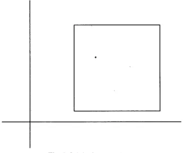
Table 1 is the result of recursive estimation developed in this

sec-tion. Figures 1-5 show the uncertainty at each step respectively.

We can see that, although the obtained uncertainties are fairly large than the informational domain, they converge to the true point as the step lncreases.

(20)

246 EMfifttyffLgfig (Y-Nft•kue eg260, 261g)

:x-

.

Fig.2 Uncertainty for s=1

(21)

Fig.4 Uncertainty for s=3

(22)

248 liNfiktsRLeJwail (P-KS•faue ag260, 261g)

Table 1. Uncertainty by the recurslve schme.

ITERATION

C, C2

MIN

_MAX

MIN

_MAX

o 2,OOO 6.000 O.500 4.500 1 pnnn"-vvv _6.000 _2.377 _3.704 2 2,OOO 4.178 2.377 3.704 3 2.000 4.178 2.679 3.704 4 2.000 4.178 2.679 3.464 5 2.394 4.178 2.679 3.464 6 2.394 3.507 2.679 3.464 7 2.610 3.507 2.679 3.464 8 2.610 3.373 2.679 3.464 9 2.610 3.373 2.679 3.464 10 2.610 3.373 2.679 3.464 20 2.968 3.171 2.864 3.042 30 2.968 3.159 2.864 3.042 40 2.968 3.159 2.864 3.042 50 2.968 3.159 2.934 3.042 60 2.974 3.159 2.934 3.042 70 2.974 3.159 2.934 3.042 80 2.974 3.014 2.969 3.015 90 2.974 3.014 2.969 3.015 100 2.974 3,O14 2.969 3.015 200 2.986 3.007 2.997 3.015 300 2.988 3.007 2.997 3.015 400 2.991 3.005 2.997 3.015 500 2.994 3.005 2.997 3.015 600 2.994 3.005 2.997 3.005 ' 700 2.994 3.005 2.997 3.005 800 2.994 3.001 2.997 3.005 900 2.994 3.001 2.997 3.005 1000 2.996 3.001 2.998 3.004

(23)

5. Conclusions

In this paper, the identification problem with deterministic

uncer-tainty was discussed. The exact unceruncer-tainty set was formulated by

the intersection of convex sets. Next, for the uncertainty expressed by orthotopes, it was shown that the solution set was given by the

solu-tion of LP or NLP problems. A recursive scheme was proposed, where the uncertainty was approximated by an orthotope whose

edges are parallel to the axes at every stage.

References

Akaike, H (1981) Modern development of statistical methods, in Trends and thogress in Systems ldentification (ed. by Eykhoff), Pergamon Press. Cox, D.R. and D.V. Hinkley (1974) Theoretical Statistics, Chapman and Hall, London.

Eykhoff, P. (1974) System Identification: Parameter and State Estimation, J.

Wiley and Sons, New York.

Fogel, E. and Y.F. Huang (1982) On the value of information in system

identification-bounded noise case, Automatica, Vol. 18, No.2, pp.229-238.

Kurzhanski, A.B. (1988) Identification-a theory of guaranteed estimates, WP-88-55, IIASA Worhing Paper, IIASA, Laxenburg, Austria.

Lozano-Leal, R. and R. Ortega (1987) Reformulation of the parameter identificaqtion problem for systems with bounded disturbances, Automatica, Vol.23, No.2, pp.247-251.

Norton, J.P. (1987) Identification and application of bounded-parameter models, Automatica, Vol.23, No.4, pp.497-507,

Rockafellar, R.T. (1970) Convex Analysis, Princeton University Press.

Walter, E. and H. Piet-Lahanier (1989) Exact recursive polyhedral scription of the feasible parameter set for bounded-error models, IEEE Trans. Autonzatic Control, VoL34, No.8, pp.911-915.