2003, Vol. 46, No. 4, 503-522
REGENERATIVE CYCLE METHOD IN M/G/1 WITH MANY VACATION RULES
Toshinao Nakatsuka
Tokyo Metropolitan University
(Received October 22, 2002; Revised April 10, 2003)
Abstract This paper gives a new method to derive the time average distribution of queue length in the model M/G/1 with many vacation rules. We extract many kinds of regenerative cycles of the well-known regenerative processes from the queue length process of the model by using the method shown by Fuhrmann and Cooper. The time average of the original model is represented by the combination of the time averages of such regenerative processes. We find this combination in various models, e.g., the model with setup time, the special decrementing service system, pure limited service system, feedback system and so on. We show a recursive calculation formula for moments.
Keywords: Queue, regenerative cycle method, M/G/1, vacation, pure limited service system
1. Introduction
The M/G/1 is the fundamental queueing model and its many properties have been discov-ered. The variants of M/G/1 are also, sometimes more, important in real application to many fields of operations research. These variants give rise to many problems which we must solve. This paper was stimulated from the study of the queue length of the M/G/1 with server vacations. In the setting of early authors the vacation begins only when there is no customer in the system(e.g., [3]). They(see Takagi’s book[20] or Doshi’s servey[5]) studied the model with multiple vacation or the model with N-policy, and derived the probability generating function(PGF) of the queue length at the departure epoch or at an arbitrary time as the decomposition form. Afterwards some authors considered the case that the server takes a vacation even when there is a customer in the system. Particularly Fuhrmann and Cooper[7] obtained the generalized decomposition theorem about queue length in the model with one type of vacation. Shanthikumar[16] pointed out that such decomposition holds for vacations other than an ordinary vacation. However their technique has not prevailed. For example, Takagi([20] p.202) introduced most results in the gated service system or other important models by using other technique. Wortman and Disney[23] used the Markov renewal process embedded in the model. One reason is thought to be that the generalized decomposition theorem is available for the model with only one type of vacation. Therefore, the applicable models are limited.
When we consider the real application, the analysis of the model with several vacation rules is necessary. In such model their decomposition theorem is not useful. Really, if we regard the idle period in M/G/1 as a vacation, it is essentially different with the ordinary vacation which is independent of the arrival epochs. So it is difficult to deal with these vacations all together as one type of vacation. The model with two or three types of vacation has been discussed individually, e.g., gated service system with multiple vacation([17]),
threshold policy model of [26], etc. This paper considers Fuhrmann and Cooper’s technique in such model and obtains the time average PGF of the queue length yt for some variants of M/G/1.
Fuhrmann and Cooper defined the vacation customers and their offsprings whom one vacation generates. From any sample path of the model they extracted the time domain consisting of one vacation period and service periods of its customers and offsprings. This paper regards their time domain as one cycle of the regenerative process. Therefore if the model has many vacation rules, it generates many types of such regenerative cycles. We represent the time average PGF of yt by the combination of the PGF’s of the regenerative processes which the vacations of this model generate.
Conversely speaking, we can make new model by combining the regenerative processes. As the fundamental regenerative processes, this paper chooses M/G/1 with N-policy and
M/G/1 with multiple vacation. The former is the regenerative process generated by
N-policy vacation and the latter is the regenerative process generated by the ordinary vacation. Successive occurrence of the regenerative cycles of these two kinds of regenerative processes generates many interesting variants of M/G/1. Since the time average PGF’s of these two models are well known, we can calculate PGF of the variant model through the combination of the PGF’s of these two fundamental models. We illustrate our technique in many exam-ples, e.g., model with setup time, special decrementing service system, pure limited service system, feedback system and so on. Moreover Theorem 4.1 which is our main theorem is not restricted only to the combination of the fundamental regenerative cycles. If we obtain the PGF’s of complicated regenerative processes, we can obtain the PGF of more complicated model by combining these regenerative processes. However, since one purpose of this paper is to show the possibility of easy calculation, we do not deal with the extremely entangled example.
In order to consolidate the foundations, we must discuss strictly and clarify the con-dition. This paper uses the M/G/1 with multiple vacation as an important fundamental regenerative process. The cycle length between regeneration points in this model has the lattice distribution for special distributions of service and vacation and for a special initial condition in spite of the Poisson arrival, so that it has not the limiting distribution for such initial state. Moreover the stability of the model is not directly related with Theorem 4.1. Therefore we focus our attention to the time average.
The technique of this paper derives the time average PGF of the queue length for many models. We can obtain probabilities and moments of its probability measure by differenti-ating it. The representation of the combination is also useful for this calculation. However the differentiation of some fundamental PGF’s is necessary and it is laborious if we try it directly. In last section we improve the classical recursive calculation method.
2. M/G/1 With Vacations
2.1. The customers generated by a vacation
Before discussing the general theory in sections 3 and 4, this section defines a time domain in a queueing system which consists of the vacation interval and the service times of customers generated by its vacation. This time domain is the typical example of the time domain discussed in the general theory. Moreover, we use it as a fundamental regenerative cycle in later sections. Every queueing system in our examples has a single server. Our system starts at the epoch zero with an idle state. Let ytbe the number of customers in the system at a time epoch t ∈ [0, ∞). The server sometimes takes vacations. In this paper we regard
an idle period as a vacation, too. So any epoch on the total time domain [0, ∞) belongs to a service period on which the server is working or to a vacation period on which the server is not working. The customers arrive according to Poisson process with constant intensity
λ. On the other hand the service times are i.i.d. with the distribution function B(x) and
they are independent of the arrival process. Let b and B∗(s) be the mean and the Laplace Stieltjes transform(LST) of B(x) respectively. We put ρ = λb. The service discipline is the nonpreemptive LIFO(Last In, First Out). In many cases the stochastic behavior of yt is identical among nonpreemptive LIFO, FIFO, service in random order or other similar service disciplines, so that we can apply our results to these cases.
The various kinds of vacation rules are possible as is shown in [6, 16]. Particularly with respect to the arrivals during a vacation we can consider balking, reneging and other rules on the vacation. However the examples in this paper use the only following two kinds of vacations.
1. The ordinary vacation. Once this vacation begins, its length of vacation period is determined independently of the arrival process and service times. All customers who arrive during the vacation period continue to stay in the system until the end of this period.
2. N-policy vacation. The N customers arrive during this vacation. This vacation ends when the last customer among these N customers arrives. As the special case, the idle time interval in the ordinary M/G/1 is the vacation period with 1-policy.
We denote the kth vacation after the starting epoch zero by the notation Vk. In [7] the customers who arrive during the vacation Vk are called the vacation customers and their set is denoted by Ik
0. To define strictly, we assume that the customer who happens to arrive
just at the beginning of Vk does not belong to Ik
0 and the customer who happens to arrive
just at the end of Vk belongs to Ik
0. That is, the vacation period is the half open interval
with the form (a, b], if it is not interrupted. The important example of the former case is the model with setup time and the important example of the latter case is the N-policy rule.
The customers who arrive while the members of Ik
i−1 are being served are called the ith generation offsprings and their set is denoted by Ik
i. We put Gk ≡ ∪∞i=0Iik. Two different vacations do not duplicate, so that Gi∩ Gj is the null set for i 6= j.
In section 4 we define the time domain Jk(⊂ (0, ∞)) generally. As its typical example, this section considers the union of the time interval of Vk and the service periods on which the customers in Gk are served. If Jk is so, in many variants of M/G/1 we often find that a certain vacation Vk+1 starts before J
k ends. In this case the remaining customers in Gk wait until Jk resumes. We should note that the Jk resumes after the completion of Jk+1 because of LIFO discipline. Under the assumption of Poisson arrival the probability behavior of the queue length on the Jk is not influenced by the interruption of Jk+1. If this is guaranteed, we can consider the case that the vacation begins in the middle of the service. Let lk be the number of customers staying at the beginning of Vk. Since these customers do not belong to Gk and are served after Jk, the probability structure of yt− lk on Jk is determined only by the arrivals on it and services of customers in Gk. So we call yt− lk the regenerative cycle on Jk. If Jk is generated by a certain vacation rule, the regeneration cycle on it has the probability structure which is peculiar to this vacation rule. Since we consider the model with many vacation rules, we classify such probability structure by the type number ξk. 2.2. Examples
The following two examples have both 1-policy and an ordinary vacation. In Example 2.1 one Jk is interrupted by only one other vacation. In Example 2.2 one Jk is interrupted by several other vacations.
Example 2.1. Consider the M/G/1 with setup time. Assume ρ < 1. When there is no customer in the system, the server waits for next customer. When a customer arrives at the idle system, the server takes a setup time. After the completion of the setup time he continues to work until there is no customer in the system. Assume that the setup times are i.i.d. In this model we classify the vacations into two types. The V2k−1 is the 1-policy
vacation and it means the idle period during which the server waits for a customer. The
V2k is the ordinary vacation and it means the interval of the setup time. Clearly l
2k−1 = 0
and l2k = 1. In Figure 1, V2k−1 is the interval (a, b]. The (b, c] is the interval for setup
time and so V2k is this interval. The customer arriving at b is the customer of 1-policy
vacation V2k−1 and he is also the customer of l
2k = 1. He begins to receive service at d
because of LIFO discipline. In this model J2k−1 = (a, b] ∪ (d, e] and J2k = (b, d]. That
is, J2k−1 is interrupted by J2k. The stochastic behavior of yt on J2k−1 is independent of
that on other time domain and it is equal to the stochastic behavior of a regenerative cycle of ordinary M/G/1. Similarly the stochastic behavior of yt − l2k on J2k is equal to the
stochastic behavior of ordinary M/G/1 with multiple vacation. So we will put ξ2k−1 = 1
and ξ2k = 2 in later sections.
↑ ↑ ↑ ↑ ↑ ↑ ↑
a b c d e
V2k−1 V2k V2k+1
J2k−1 J2k J2k−1
Figure 1. Queue length yt in the model with setup time.
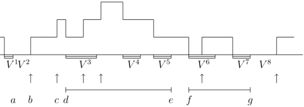
Example 2.2. Consider the M/G/1 with the pure limited vacation rule. In this model, the server takes one ordinary vacation after each service. In Figure 2, V1, V3, · · · , V7 are
such ordinary vacations. The V2 and V8 are 1-policy vacations. The server waits for next
customer after returning from vacation V1. The customer arriving at b begins to receive
the service at once, its service ends at d and the server takes the vacation V3. From LIFO
discipline the customer arriving at c begins to receive the service at e. The time domain generated by 1-policy vacation V2 is (a, d] ∪ (e, f ]. Therefore the behavior of y
t on the interval (a, g] is the regenerative cycle of M/G/1 which is interrupted by two intervals (d, e] and (f, g].
V1V2 V3 V4 V5 V6 V7 V8
↑ ↑ ↑ ↑ ↑ ↑
a b c d e f g
3. Time Average
3.1. Time average and distribution at an arbitrary time
This paper considers the time average of the queue length and does not directly deal with the distribution at an arbitrary time for the following reason. The M/G/1 with multiple vacation is the fundamentally important model in this paper. However the queue length in this model has no limiting distribution in some special cases. For example, let’s consider the case that both the service time and the vacation time take the values of integer with probability one. If the first vacation begins at an epoch of integer, e.g., 0, this vacation ends at an epoch of integer. Since any time epoch belongs to the vacation period or the service period, all vacation times and all service periods begin at epochs of integer in spite of the arrival process. Conversely if the first vacation begins at an epoch of non-integer, all vacation times begin at epochs of non-integer. That is, the influence of the fixed initial state is eternal. Moreover if the first vacation begins at an epoch of integer, the customers leave the system only at epochs of integer, so that the distribution of queue length immediately before an integer is different from that immediately after this integer epoch. Thereby there is not the limiting distribution of the number of customers on the continuous time parameter domain for a fixed initial condition.
The beginning of the vacation in M/G/1 with multiple vacation is the regeneration point. In above example the differences between these points are integers. That is, the renewal interval has the lattice distribution to which much of the regenerative theory is not applicable(see Asmussen[1]). On the other hand any regenerative process becomes stationary if we add the special initial condition(see [25, p.110]). From this fact most authors(e.g.,[7, 9, 12, 19]) used the term ”distribution at an arbitrary time”. We must take cares. This term does not imply the stability in the sense of the existence of the limiting distribution with a fixed initial state. Our result holds also for the model with the fixed initial state or even for non-regenerative process, so that we use the term ”time average”. As is well known, if a process is stationary and ergodic, or if it is the stationary regenerative process, its distribution at an arbitrary time is identical to the time average.
3.2. Time average and regenerative process
Let (Ω, σ(Ω), P ) be the basic probability space. Let yt be the nonnegative integer-valued process which we want to analyze. We use abbreviation w.p.1 for ”with probability one in
P ”. We define the time average of the set u(⊂ {0, 1, 2, · · · }) by T A(u) = lim T →∞T −1 Z T 0 χ(yt∈ u)dt w.p.1, (3.1)
if the limit of the right hand side exists, where χ(A) = 1 if A holds and χ(A) = 0 otherwise. Note that this is generally not the probability of u at an arbitrary time. Moreover (3.1) does not guarantee even the uniqueness. That is, it may depend on ω ∈ Ω. When the T A(u) has the property of probability measure, its probability generating function(PGF) is defined as
Π(z) = ∞ X
j=0
T A({j})zj. (3.2)
In this paper we call this the time average PGF of yt or simply the PGF of the model. If we get Π(z), we can get T A({n}) and the moments by differentiating Π(z).
In the case that yt is the classical regenerative process with the finite mean of the cycle length, the time average of yt exists uniquely for every u. Let (0 ≤)c1 < c2 < · · · be the
regeneration points. We define
Dk = Z ck+1
ck
χ(yt∈ u)dt : k = 1, 2, · · · . (3.3)
Then the vector of two variables {Dk, ck+1− ck} is identically independently distributed for every u. It is well known([1, 25]) that the T A(u) has the property of the probability measure and is equivalent to the distribution on a cycle, i.e.,
T A(u) = E(D1) E(c2− c1)
, (3.4)
where E(•) represents the mean of the variable •. 3.3. Vacation model
The examples of this paper deal with two kinds of vacations, the N-policy vacation and the ordinary vacation. We use the PGF’s generated by these vacations without proof. They have the following forms. If, under the assumptions in section 2 the Jk generated by the
N-policy vacation is repeated independently and without interruption, it results in the
regenerative process of the ordinary M/G/1 with N-policy. We represent its time average PGF by Π(z : M/G/1/Npolicy). Particularly Π(z : M/G/1/1policy) is equal to the well known PGF Π(z : M/G/1). These PGF’s have the following forms.
Π(z : M/G/1/Npolicy) = 1 − zN N(1 − z)Π(z : M/G/1) (3.5) Π(z : M/G/1) = (1 − ρ)(1 − z)B ∗(λ − λz) B∗(λ − λz) − z (3.6)
(see [20]). Let Θk be the length of Jk. Then E(Θk) = N/{λ(1 − ρ)} is known for N-policy vacation.
In the case of the ordinary vacation with the distribution function V (x), we denote the mean and LST of V (x) by v and V∗(s) respectively. If the J
k generated by the ordinary vacation repeats independently, it becomes M/G/1 with multiple vacation. We represent this time average PGF by Π(z : M/G/1/MV (V )). As is well known, this is represented by
Π(z : M/G/1/MV (V )) = 1 − V∗(λ − λz)
λv(1 − z) Π(z : M/G/1). (3.7)
Note that this model has two kinds of regeneration points. One is to choose all beginnings of vacations and other is to choose the epoch when the customer leaves no customer behind. This paper does not use the latter regeneration points. Therefore our Jkin multiple vacation model has no service period, if no customer arrives during this vacation period, and it has the mean E(Θk) = v/(1 − ρ).
4. Theorems For Combination 4.1. General formation
We assume that we can find a sequence of the time domains {Jk : k = 1, 2, · · · } with probability one in the model which we want to analyze. We discuss generally. So, besides the time domain generated by one vacation, we can choose other time domain as Jk. For example, we will choose (d, e] in Example 2.2 as Jk in later section. The Jk satisfies the
following conditions. First, Jk has the starting epoch tk. However tk ∈ J/ k. For convenience we consider that the null set Jk is possible, so that, if Jk is not a null set, there is an open interval such that (tk, tk+²) ⊂ Jk. Secondly, Jkhas the finite end epoch ek, i.e., Jk ⊂ (tk, ek]. The ekis contained in Jkunless Jkis a null set. Thirdly, ti ≤ tj if i < j. When ti = tj(i < j), the Ji is a null set. Fourthly, the Ji∩ Jj is the null set if i 6= j. Fifthly, if Ji is interrupted by Jj, then Jj is not interrupted by Ji.
We assume that the model has the right-continuous nonnegative integer-valued process
yt. Let Θk be the length of Jk. Each Jk is classified by its type number ξk. Let Ξ be the space of values of ξk. We put lk = ytk. Let nk(t) ≡ yt− lk ≥ 0 for t ∈ Jk. Since Jk may
be interrupted by other interval, we put ˜nk(s) = nk(t) for the length s of Jk on (0, t]. The following is our essential assumption.
Assumption 4.1. The number of elements in Ξ is finite. The type ξk is determined at
tk. Once ξk is determined, the (Θk, ˜nk(s)) is distributed independently of past yt and past input containing arrival epochs, service times, vacation times and other variables. Its distribution is determined by the type number ξk. The Θk has the positive finite mean
θξ = E(Θk|ξk = ξ).
In this assumption, first we should note that the value of ξk is able to depend on the past ytor past input. Secondly although θξ must be positive, the occurrence of Θk = 0 with positive probability is possible. The Jk with Θk = 0 is a null set.
Thirdly when ξk= ξ is given, we can define the probability measure pξi by
pξi = θ−1 ξ E ³Z Jk χ(nk(t) = i)dt ¯ ¯ ¯ξk= ξ ´ (4.1)
under the condition of ξk= ξ. We put
Π(z : ξ) = ∞ X
i=0
pξizi. (4.2)
Since (4.1) is essentially identical to the distribution on Jk, from (3.4) the Π(z : ξ) is the time average PGF of the regenerative process repeating ˜nk(t)(ξk = ξ) independently.
Fourthly, since min θξ > 0 and each Jk has the finite end epoch, one Jkis not interrupted by the infinitely many other Ji’s and {tk} has no accumulation epoch. Let q be the maximum number such that Jk ⊂ [0, T ] for all k ≤ q. Then we have q → ∞ w.p.1 as T → ∞. We put
²T = T − Pq
k=1Θk and add the following two assumptions. Assumption 4.2. ∪∞
k=1Jk= (0, ∞).
Assumption 4.3. ²T/T → 0 w.p.1 as T → ∞. 4.2. Main theorem
We will show the condition for the existence of T A(j) under the above formation. Moreover we show that T A(j) has the linear representation of Π(z : ξ). For q in Assumption 4.3, let
nξ
q be the number of k such that ξk = ξ and k ≤ q. Let nξq(i) be the number of k such that
ξk = ξ, lk = i and k ≤ q. In the following assumption it is unnecessary that the limits αξ and pl
i(ξ) are constants with probability one.
Assumption 4.4. There is a finite limit αξ = limT →∞nξq/T w.p.1 for each ξ. In addition, on the set {ω : αξ > 0} except for the set with probability 0, there are numbers pli(ξ) such that pl
i(ξ) = limq→∞nξq(i)/nξq and that P∞
i=0pli(ξ) = 1 holds. For other ω ∈ Ω we put
pl
The αξ may not be unique. That is, it may depend on ω, so that the following theorem does not guarantee the uniqueness of the value of T A(j) or Π(z). We put Πl(z : ξ) = P∞
i=0pli(ξ)zi.
Theorem 4.1. Under Assumptions 4.1, 4.2, 4.3 and 4.4, the T A(j) exists with probability one and {T A(j) : j = 0, 1, · · · } constitutes a probability measure. Its PGF Π(z) is computed by Π(z) ≡ ∞ X j=0 T A(j)zj =X ξ∈Ξ αξθξΠl(z : ξ)Π(z : ξ). (4.3)
Proof. From Assumptions 4.2 and 4.3 we have
T A(j) = lim T →∞ 1 T Z T 0 χ(yt= j)dt = lim T →∞ 1 T q X k=1 Z Jk χ(yt = j)dt = lim T →∞ 1 T X ξ∈Ξ j X i=0 q X k=1 χ(ξk= ξ, lk= i) Z Jk χ(nk(t) = j − i)dt.
Thus, from Assumptions 4.1 and 4.4 we get
T A(j) = lim T →∞ X ξ∈Ξ j X i=0 nξ q T nξ q(i) nξq 1 nξq(i) q X k=1 χ(ξk = ξ, lk= i) Z Jk χ(nk(t) = j − i)dt =X ξ∈Ξ αξθξ j X i=0 pli(ξ)pξj−i. Hence (4.3) follows.
Finally we must show P∞i=0T A(i) = 1. Since ²T = T − Pq k=1Θk, we have 1 = lim T →∞ 1 T q X k=1 Θk= lim T →∞ 1 T X ξ∈Ξ q X k=1 Θkχ(ξk = ξ) = X ξ∈Ξ αξθξ. By putting z = 1 in (4.3) we find Pξ∈Ξαξθξ = P∞
i=0T A(i). Hence theorem follows. ¤
Remark 1 : The equality Pαξθξ = 1 in the proof is often used for determining αξ.
Remark 2 : The αξ and the pli(ξ) in Assumption 4.4 are constants in every example in this paper. However this is not the necessary condition. For example, consider the model such that, if the first service time after the system starts is smaller than a certain value, the system becomes M/G/1 and, if not, it becomes M/G/1 with multiple vacation. Then
T A(j) exists but it depends on the first service time.
Remark 3 : Fuhrmann and Cooper[7] stated about three-way decomposition
Π(z) = H−(z)α−(z)Π(z : M/G/1).
This is the case that ξ in our theorem takes only one type of the ordinary vacation. In this case it is written by Π(z) = Πl(z : ξ)Π(z : ξ) = Πl(z : ξ)α
4.3. Case of the regenerative process
In all applications in this paper the ytitself is the regenerative process, so that the following theorem is useful and Theorem 4.1 holds under Assumptions 4.1 and 4.2.
Theorem 4.2. Assume that the yt is the regenerative process with finite mean θy of the cycle length and that ²T = 0 at the regeneration point. Then, Assumption 4.3 holds. The
αξ and the pli(ξ) are uniquely determined for each ξ and
αξθy = E ¡
The NO of the event {ξk = ξ} in one RC ¢
, (4.4)
pl i(ξ) =
E¡The NO of the event {ξk= ξ, lk= i} in one RC ¢
E¡The NO of the event {ξk = ξ} in one RC
¢ , (4.5)
where NO and RC are the abbreviations of ”number of occurrences” and ”regenerative cycle of yt” respectively. Assumption 4.4 also holds.
Proof. Since θy is finite, Assumption 4.3 holds. Let T1 < T2· · · be regeneration points. Let
mξi be the number of occurrences of Jk with ξk = ξ in the ith regenerative cycle of yt. This
mξi is identically independently distributed. Hence (4.4) follows from
αξ= lim T →∞ 1 Tn ξ q = limj→∞ j Tj+1 1 j j X i=1 mξi. Similarly pl
i(ξ) is constant and (4.5) holds. By the monotone convergence theorem we have P∞
i=0pli(ξ) = 1, so that Assumption 4.4 holds. ¤
5. Examples; Setup Time
This paper takes up several examples with one class of Poisson arrivals with intensity λ. This section considers two models with setup.Let V (x) and v be the distribution function of the length of the setup time and its mean respectively.
In the ordinary setup model in Example 2.1, we choose 1 and 2 as the values of the type ξ. The ξ = 1 represents the 1-policy vacation V2k−1 and ξ = 2 represents the ordinary
vacation V2k which means setup time with V (x). Then θ
1 = {λ(1−ρ)}−1and θ2 = v/(1−ρ).
Clearly the queue length ytis the regenerative process. As the regeneration point we choose the epoch when the customer leaves no customer behind. One regenerative cycle consists of two time domains J2k−1 and J2k, where Ji is the time domains generated by Vi. Clearly the mean θy of cycle length satisfies θy = θ1+ θ2, so that αξ and pli(ξ) of Assumption 4.4 are uniquely determined from Theorem 4.2. Clearly α1 = α2. Since α1θ1+ α2θ2 = 1, we get
α1 = α2 = λ(1 − ρ)/(1 + λv). On the other hand there is no customer at the beginning of
J2k−1, so that pl0(1) = P r{lk = 0|ξk = 1} = 1. There is one customer at the beginning of
J2k so that pl1(2) = P r{lk = 1|ξk= 2} = 1. From Theorem 4.1 the time average PGF of the queue length yt of this model is given by
Π¡z :M/G/1/Setup¢ = 1 1 + λvΠ(z : M/G/1) + λv 1 + λvzΠ ¡ z :M/G/1/M V (V )¢. (5.1)
This is identical to the equation of [20]p.131. The differential Π(n)¡z :M/G/1
/Setup ¢
is easily obtained from (5.1), if we know Π(n)(z : M/G/1)
and Π(n)¡z :M/G/1
/M V (V ) ¢
which are discussed in last section. Similar arguments about differentials hold in equations in this and later sections.
In the same way we can extend the type ξ = 1 to N-policy. Its result is Π¡z :M/G/1/Npolicy /Setup ¢ = N N + λvΠ ¡ z :M/G/1/Npolicy¢+ λv N + λvz NΠ¡z :M/G/1 /M V (V ) ¢ (5.2)
(also see [20]p.135). We get θy = θ1+ θ2 = (N + λv)/{λ(1 − ρ)}.
Secondly let’s consider the model with multiple vacation and setup time. If the server finds customers at the end of the vacation, he begins to serve them after the setup time. If not, he takes another vacation. We choose 1 and 2 as the values of ξ. Both are the types of the ordinary vacation. The ξ = 1 means the vacation of real model. Let V1(x)
be its distribution function. Let v1 and V1∗(s) be its mean and LST respectively. Then
θ1 = v1/(1 − ρ). The type ξ = 2 means the setup time with V (x). As the regeneration point
we choose every beginning of the vacation of type ξ = 1. Then θy < θ1+ θ2 < ∞ so that
Theorems 4.1 and 4.2 hold. We have α1 : α2 = 1 : 1 − V1∗(λ). Since α1θ1+ α2θ2 = 1, we get
α1 = 1 − ρ β and α2 = (1 − ρ)(1 − V∗ 1(λ)) β
where β = v1+ v(1 − V1∗(λ)). There is no customer at the beginning of the vacation with
ξ = 1, so that Πl(z : ξ = 1) = 1. The Πl(z : ξ = 2) is equal to the PGF of the number of the customers arriving during the vacation with ξ = 1 on the condition that at least one customer arrives, so that Πl(z : ξ = 2) = {V∗
1(λ − λz) − V1∗(λ)}/(1 − V1∗(λ)). Hence Π¡z :•/M V (V/Setup 1)¢= v1 β Π ¡ z :M/G/1/M V (V1)¢+ v β ¡ V∗ 1(λ − λz) − V1∗(λ) ¢ Π¡z :M/G/1/M V (V )¢, (5.3)
where • is the abbreviation of ”M/G/1”. We get θy = θ1+ {1 − V1∗(λ)}θ2 = β/(1 − ρ). By
the further calculation of (5.3) we find that it is equal to Qs(z) of [2, p.280]. 6. Examples: Simple State Dependent Vacation
To M/G/1/Npolicy and M/G/1 with multiple vacation this section adds the condition that the server takes an ordinary vacation only when the number of waiting customers at the epoch of the completion of the service is one. That is, lk = 1 for this vacation. We denote this distribution function, its mean, its LST and its type number by V (x), v, V∗(s) and
ξ = 2 respectively. If Theorem 4.1 holds, we can represent
Π¡z :•/Npolicy /lk=1 ¢ = Nα1 λ(1 − ρ)Π ¡ z :M/G/1/N policy ¢ + vα2 1 − ρzΠ ¡ z :M/G/1/MV (V )¢ (6.1)
for this variant of M/G/1/Npolicy and Π¡z :•/M V (V/l 1) k=1 ¢ = v1α1 1 − ρΠ ¡ z :M/G/1/M V (V1)¢+ vα2 1 − ρzΠ ¡ z :M/G/1/MV (V )¢ (6.2)
for this variant of M/G/1/MV (V1).
This section considers only (6.1) with N = 1 for the space saving. The ξ = 1 corresponds to the vacation of 1-policy. We consider two cases. First we assume that the server takes a vacation of ξ = 2 only once during one interval such as yt > 0. As a regeneration point we choose the epoch when the customer leaves no customer behind. Then θy < θ1+ θ2 =
(1 + λv)/{λ(1 − ρ)} < ∞, so that αξ and pli(ξ) of Assumption 4.4 are uniquely determined from Theorem 4.2. The server takes the vacation of ξ = 2, if at least one customer arrives
during the first service time. So we have α1 : α2 = 1 : 1 − B∗(λ). From α1θ1+ α2θ2 = 1, we get λ−1α 1+ vα2 = 1 − ρ. Hence α1 = λ(1 − ρ) β and α2 = λ(1 − ρ)(1 − B∗(λ)) β , where β = 1 + λv(1 − B∗(λ)). Therefore Π¡z :M/G/1/lk=1 ¢= 1 βΠ(z : M/G/1) + λv(1 − B∗(λ)) β zΠ ¡ z :M/G/1/M V (V )¢. (6.3)
Secondly we assume that the server always takes the vacation of ξ = 2, if he finds exactly one waiting customer at the end of the service of the customer. The regenerative cycle consists of the Jk of 1-policy vacation with ξ = 1 and the time domains Jk+1, Jk+2, · · · generated by ordinary vacations with ξ = 2. If a customer arrives during the interval from the beginning of the ordinary vacation and to the end of one service immediately after this vacation, the server takes next ordinary vacation. Hence the probability that the server takes m vacations during one period such as yt> 0 is
½
B∗(λ) if m = 0
©
1 − B∗(λ)ªV∗(λ)B∗(λ)©1 − V∗(λ)B∗(λ)ªm−1 if m > 0. The mean of m is calculated as
E(m) = 1 − B
∗(λ)
V∗(λ)B∗(λ).
Therefore from Wald’s equation(e.g., [25]p.98) we find θy = θ1 + E(m)θ2 < ∞. We have
α1 : α2 = 1 : E(m). Since λ−1α1+ vα2 = 1 − ρ, we get
α1 = λ(1 − ρ) 1 + λvE(m) and α2 = λ(1 − ρ)E(m) 1 + λvE(m) . Hence Π¡z :M/G/1/l k=1 ¢ = 1 1 + λvE(m)Π(z : M/G/1) + λvE(m) 1 + λvE(m)zΠ ¡ z :M/G/1/M V (V )¢. (6.4)
7. Base Model Interrupted By Regenerative Cycles
The regenerative cycle in Example 2.1 begins with a vacation of 1-policy and the Jkgenerated by this vacation is interrupted by one ordinary vacation. Similar interruption is seen in any model in sections 5 and 6. Moreover in Example 2.2 the Jk with 1-policy vacation is interrupted by the interval (d, e] and followed by (f, g]. The probability structures on these intervals are the same if we ignore yd and yf. Roughly speaking, in these models the well known regenerative process which we call the base model is interrupted by other regenerative cycles and resumes without sustaining any damage to its probability structure. The yt in these models is also a regenerative process whose regeneration point is the beginning of the cycle of the base model. If we give the interrupting regenerative cycle the type number ξ, this style has the PGF with the following form from Theorem 4.1.
We can construct many models whose PGF’s are obtained by this equation, if we know Πbase(z) and Π(z : ξ). Moreover, by using (7.1) repeatedly, we can obtain the PGF’s for many complicated models.
In the examples in previous sections, Π(z : ξ) is the PGF (3.7) of M/G/1 with multiple vacation. In this case we have
Π(z) = αbaseθbaseΠbase(z) +
vαξ 1 − ρΠ l(z : ξ)Π¡z :M/G/1 /M V (V ) ¢ . (7.2)
Typical application of (7.2) is the single vacation. The server takes a vacation with V (x) at the end of a regenerative cycle of the base model and the cycle of M/G/1/MV (V ) begins. This cycle is not interrupted by other interval. Here we assume that, if he finds a customer on return from the vacation, he begins services and takes the vacation again at the end of this busy period. If he finds no customer on return from the vacation, the new cycle of the base model begins. The PGF of this model is represented in the form of (7.2). In this case
αbase : αξ = 1 : V∗(λ) P∞
i=0(i + 1)(1 − V∗(λ))i = 1 : V∗(λ)−1 and Πl(z : ξ) = 1. Therefore
αbase = (1 − ρ)V∗(λ)/ ¡ θbase(1 − ρ)V∗(λ) + v ¢ and Π(z) = (1 − ρ)V∗(λ)θbase (1 − ρ)V∗(λ)θbase+ vΠbase(z) + v (1 − ρ)V∗(λ)θbase+ vΠ ¡ z :M/G/1/M V (V )¢. (7.3)
When Πbase(z) = Π(z : M/G/1), the (7.3) becomes the equation (4.3) of [5].
It is possible to extend (7.2) to the independent selection of ordinary vacations which have the different distribution functions V1(x), · · · , Vp(x). Let vi be the mean of Vi(x). Assume that, when the server takes a vacation, he chooses Vi(x) with probability δi and takes a corresponding vacation. If this selection is i.i.d. and independent of other variables, the PGF of the queue length at the beginning of the vacation is the same among these vacations so that we denote it by Πl(z : ξ = 0). Then we have the following form from Theorem 4.1.
Π(z) = αbaseθbaseΠbase(z) + α0Πl(z : ξ = 0)
p X i=1 δivi 1 − ρΠ ¡ z :M/G/1/M V (V i) ¢ . (7.4)
The case of vp = 0 is possible in (7.4) or Theorem 4.1, so that we can deal with the Bernoulli schedule where the server takes a vacation with a certain probability δ(see [20, p.246]). 8. Examples: Pure Limited Service System
This section considers the model where the server takes an ordinary vacation at each end of the service, even if there is no customer at this epoch. Such model is called the pure limited service system([11, 20]). Let V (x) be the distribution function of the length of this ordinary vacation. Let v and V∗(s) be its mean and LST. As the base model we choose
M/G/1, M/G/1/Npolicy, M/G/1 with setup time, M/G/1/MV (V1) and so on. We denote
these variants by M/G/1/Npolicy/P L(V ), M/G/1/MV (V1)/P L(V ) and so on.
First we will consider M/G/1/MV (V1)/P L(V ). We can write
Π¡z :M/G/1/M V (V1)/P L(V )¢= α1v1 1 − ρΠ ¡ z :M/G/1/M V (V1)¢+ α2v 1 − ρΠ l(z)Π¡z :M/G/1 /M V (V ) ¢ .
One vacation V accompanies one service, so that α2 = λ. Since (α1v1+ α2v)/(1 − ρ) = 1,
the beginning of the vacation of V and let ak be the number of customers arriving during this vacation. Then lk+ ak is stochastically equal to the number of customers immediately after the service in M/G(B ∗ V )/1/MV (V1). Therefore
Πl(z) = Π¡z :M/G(B∗V )/1 /M V (V1) ¢. V∗(λ − λz). Consequently we get Π¡z :M/G/1/M V (V1)/P L(V )¢= 1 − ρ − λv 1 − ρ Π ¡ z :M/G/1/M V (V1)¢ + λv (1 − ρ)V∗(λ − λz)Π ¡ z :M/G(B∗V )/1/M V (V1) ¢Π¡z :M/G/1/M V (V )¢, where Π¡z :M/G(B∗V )/1/M V (V ) ¢= (1 − ρ − λv){1 − V∗(λ − λz)}B∗(λ − λz)V∗(λ − λz) λz{B∗(λ − λz)V∗(λ − λz) − z} , from the equation (4.3).
Particularly when V1 = V , we put
Π(z : ξP L) ≡ Π¡z :M/G/1/M V (V )/P L(V )¢ = (1 − ρ − λv){B ∗(λ − λz) − z} (1 − ρ){B∗(λ − λz)V∗(λ − λz) − z}Π(z : M/G/1/MV (V )) = (1 − ρ − λv)B∗(λ − λz)(1 − V∗(λ − λz)) λv{B∗(λ − λz)V∗(λ − λz) − z} . (8.1) This is equal to the equation calculated from [20, (6.103)].
We will try to use (7.1) by inserting (8.1) to other base model. Let’s note that, since the model has the nonpreemptive LIFO discipline, the length of the interval from the end of the service of the base model to the epoch at which the base model begins again, e.g., the interval (d, e] or (f, g] in Example 2.2, is stochastically identical. That is, it is stochastically equal to the length of the regenerative cycle in M/G(B ∗ V )/1/MV (V ), so that its mean is
v/(1 − ρ − λv). We choose this interval as one Jk. The probability structure of yt− lk on this interval is equal to a regenerative cycle of M/G/1/MV (V ) with pure limited vacation rule, i.e., M/G/1/MV (V )/P L(V ) of (8.1). We give this interval the type number ξP L.
Let’s consider the model in which a base model is interrupted by the Jk with type ξP L. Let Πbase(z) and θbase be the PGF of the base model and the mean of its cycle length respectively. Since the mean of the number of customers arriving during a regenerative cycle in the base model is λθbase, the mean θy of the regeneration cycle of yt, e.g., (a, g] in Example 2.2, is given by θy = θbase+ λθbase v 1 − ρ − λv = 1 − ρ 1 − ρ − λvθbase, so that we assume ρ + λv < 1. Hence the (7.1) is written in the form:
Π(z :base
/P L(V )) = αbaseθbaseΠbase(z) + αP L
v
1 − ρ − λvΠ
Since αbase : αP L = 1 : λθbase and αbaseθbase+ αP Lv/(1 − ρ − λv) = 1, we have
αbaseθbase= 1 − ρ − λv
1 − ρ and αP L = λ
1 − ρ − λv 1 − ρ .
The regenerative cycle ξP L begins at every end of service of the base model. Therefore Πl(z : ξP L) is the distribution of the queue length immediately after the departure epoch in the base model. From Burke’s theorem and Wolff’s PASTA, we have Πl(z : ξP L) = Π
base(z). Hence (8.2) becomes Π(z) =³1 − ρ − λv 1 − ρ + λv 1 − ρΠ(z : ξ P L)´Π base(z) (8.3) = (1 − ρ − λv){B∗(λ − λz) − z} (1 − ρ){B∗(λ − λz)V∗(λ − λz) − z}Πbase(z). (8.4) For example Π(z : M/G/1/P L(V )) = (1 − ρ − λv)(1 − z)B ∗(λ − λz) B∗(λ − λz)V∗(λ − λz) − z . (8.5) 9. Examples: Decrementing Service System
Takagi[20], Bischof[2] etc. discussed the decrementing service system where the server mem-orizes the queue length at the end of the vacation. In this section we assume that the server observes the system at the beginning of the vacation. That is, when the ordinary vacation
Vk of this rule starts, the server memorizes the value l
k(> 0) and takes a rest. Returning from that vacation, he continues to work until the number of customers decreases to lk− 1 and takes another vacation Vk+1. This is repeated until there is no customer in the system. Assume that these vacations have the same distribution function V (x) with mean v and LST V∗(s). We give them the type number ξV. If we consider such model as the variation of the base model, its PGF has the form:
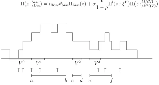
Π(z :base/Dec) = αbaseθbaseΠbase(z) + α
v 1 − ρΠ l(z : ξV)Π¡z :M/G/1 /M V (V ) ¢ . (9.1) V0 V1 V2 V3 ↑ ↑ ↑ ↑ ↑ ↑ ↑ ↑ a b c d e f
Figure 3. Queue length yt in M/G/1/3policy with decrementing service rule.
First we choose M/G/1/Npolicy as the base model. We assume that the server takes the first vacation of type ξV when the Nth customer in N-policy vacation arrives. Figure 3 illustrates the case of N = 3. The V0 is the 3-policy vacation. The server takes the
first vacation at a and (a, b) is the interval generated by this vacation. Similarly (c, d) and (e, f ) are the intervals generated by the second and the third vacations respectively. The probability structure of the remaining parts is equal to M/G/1/Npolicy. Clearly l1 = 3, l2 = 2
and l3 = 1.
After the N-policy vacation he takes N vacations with lk = N, N − 1, · · · , 1. The mean of the length of a regenerative cycle of ytis θy = N(1+λv)/{λ(1−ρ)} < ∞, so that Theorem 4.2 holds. We have αbase : α = 1 : N, θbase = N/{λ(1 − ρ)} and Πl(z : ξV) = N−1
PN i=1zi. From these equations we get
Π¡z :•/Npolicy /Dec ¢ = 1 1 + λvΠ ¡ z :M/G/1/N policy ¢ + λv N(1 + λv) z − zN +1 1 − z Π ¡ z :M/G/1/M V (V )¢. (9.2)
Next we choose M/G/1/MV (V1) as the base model. When customers arrive during a
vacation with V1(x), the server takes first vacation of type ξV at the end of the vacation
with V1(x) and takes other vacations according to the decrementing vacation rule. In (9.1)
the ratio αbase : α = 1 : λv1 holds and αbasev1/(1 − ρ) + αv/(1 − ρ) = 1. One and only one
vacation of type ξV with l
k = j is generated in one regenerative cycle of yt if more than or equal to j customers arrive during the vacation with V1(x). Let p customers arrive during
a vacation with V1(x). Then,
Πl(z : ξV) = ∞ X i=0 pl i(ξV)zi = 1 λv1 ∞ X i=1 P r(p ≥ i)zi = 1 λv1 ∞ X i=1 ∞ X j=i P r(p = i)zi = z λv1(1 − z) ∞ X j=1 (1 − zj)P r(p = j) = z λv1(1 − z) (1 − V∗ 1(λ − λz)). Consequently Π¡z :•/M V (V/Dec 1)¢= 1 1 + λvΠ ¡ z :M/G/1/M V (V1)¢+vz © 1 − V∗ 1(λ − λz) ª (1 + λv)v1(1 − z) Π¡z :M/G/1/M V (V )¢. (9.3)
10. Examples: Bernoulli Feedback
The results in this paper can be easily extended to the model with Bernoulli feedback. In this model the customer joins the queue immediately after the completion of his each service with probability 1 − σ and departs forever with probability σ. Let BF(x) be the distribution of the total service time of one customer. Then its LST B∗
F(s) is given by
B∗ F(s) =
σB∗(s) 1 − (1 − σ)B∗(s)
and the mean of BF(x) is b/σ(see [20]p.50). In Bernoulli feedback the distribution of the queue length is the same among FIFO, nonpreemptive LIFO, service in random order etc. So we consider the case that the customer receives his all services without interruption by other customer and that the service discipline is the nonpreemptive LIFO. Therefore,
unless other vacation interrupts the continuity of his services, we can extend the previous all examples to the feedback model by replacing B(x) with BF(x).
Here we consider three variants of the Bernoulli feedback. First, we consider the case that, if there is no other customer at the end of a service of a customer, the server takes a rest until there exist N(> 1) customers in the system. That is, if that customer requires another service, he must wait for arrivals of other N − 1 customers. If not, the server waits for N new customers. We choose 1 and 2 as the values of ξ. The ξ = 1 represents the (N − 1)-policy vacation and the ξ = 2 represents N-policy vacation. As the regeneration point of yt we choose the beginning of the vacation of N-policy. The type is determined by whether the last customer requires another service or not. If H is the number of occurrences of the vacation of the (N − 1)-policy in a regenerative cycle, its probability is given by
P r{H = j} = σ(1 − σ)j. Hence the mean θ
y of cycle length is finite from Wald’s equation. We have α1 : α2 = 1 − σ : σ. From θ1α1+ θ2α2 = 1, we have (N − 1)α1+ Nα2 = λ(1 − λb/σ).
Hence we get
Π(z : F eedback1) =(N − 1)(1 − σ)
N − 1 + σ zΠ(z : M/G(BF)/1/(N − 1)policy)
+ Nσ
N − 1 + σΠ(z : M/G(BF)/1/Npolicy). (10.1)
Second, the customer receives only one service. However, if he can find no customer behind at the completion of his service, he receives another service with probability 1 − σ. The interval from the beginning of this additional service to the next service completion time where its customer finds no customer behind is stochastically equal to the busy period of M/G/1. Its PGF Π(z : busy) satisfies
Π(z : M/G/1) = 1 − ρ + ρΠ(z : busy),
which is the simple case of Theorem 4.1. Hence the PGF of our second variant of the original feedback system is written as
Π(z : F eedback2) = α1θbaseΠbase(z) + α2
b
1 − ρΠ(z : busy). (10.2) When the base model is M/G/1, we have α1+ α2ρ = λ(1 − ρ) and
Π(z : F eedback2) = α1+ α2
λ(1 − ρ)Π(z : M/G/1) − α2
λ . (10.3)
If there is no restriction on the number of feedbacks, then α1 : α2 = 1 : (1 − σ)/σ. We have
Π(z : F eedback2) = 1
σ + (1 − σ)ρΠ(z : M/G/1) −
(1 − σ)(1 − ρ)
σ + (1 − σ)ρ .
Thirdly we will consider the pure limited service system with Bernoulli feedback. We assume that the sequence of services of one customer is not interrupted by the service of other customer. If a customer receives the n services, he experiences n − 1 vacations of the server with V (x) from the beginning of his service to his departing epoch. The LST of the distribution of this time length is given by
B∗
pure(s) =
σB∗(s)
with the mean (b + v − σv)/σ. If we regard this as the service period, our model becomes the ordinary pure limited service system. Therefore by replacing B∗(s) in (8.4) by B∗
pure(s) we can obtain the PGF of the feedback model with the pure limited vacation rule for each corresponding base model.
Wortman et al.[24] considered the case that the server takes vacation V with probability
δ immediately after each service. Such vacation is equal to the vacation V0 with the LST
V∗
0(s) = 1 − δ + δV∗(s) and the mean v0 = δv. We substitute this into V∗(s) of (10.4) and
put
B∗ δ(s) =
σB∗(s)
1 − (1 − σ)B∗(s)(1 − δ + δV∗(s)).
While they do not write their model in detail, their model is considered to be our ξP L from the matrix Ddv of [24]. So we will substitute Bδ∗(s) to (8.4). Then we obtain their equation (10) with different coefficient. Their equation (10) does not satisfy limz→1Ψd(z) = 1. 11. Appendix: Probabilities and Moments
Differentiating PGF, we can obtain probabilities and moments of its probability measure. However to differentiate the equation of PGF directly is very laborious. This is the serious problem for us, because our final aim is not PGF but these values. The technique which the early authors showed were laborious or vaguely represented, so this section shows the easy recursive calculation.
11.1. Calculation of probabilities
The PGF Π(z) appearing in this paper has the form Π(z) = D(z)/C(z) where C(1) =
D(1) = 0 and C(0) 6= 0. We write
C(z)Π(z) = D(z). (11.1)
By differentiating both sides n times, we get n X i=0 µ n i ¶ C(n−i)(z)Π(i)(z) = D(n)(z).
Hence the following recursive relation holds.
Π(n)(0) = 1 C(0) n − n−1 X i=0 µ n i ¶ C(n−i)(0)Π(i)(0) + D(n)(0) o . (11.2)
From this relation we can obtain the probability pn = Π(n)(0)/n! or time average of (3.1). The (11.2) is useful for the complicated PGF like Π(z : ξP L) of (8.1). In M/G/1 some authors([4, p.214][8, p.232][13]) recommended to use the transition matrix of the Markov chain. If we use (11.2) in this model, we put C(z) = B∗(λ − λz) − z, D(z) = (1 − ρ)(1 −
z)B∗(λ − λz) and c
n = (−λ)nB∗(n)(λ). Then C0(0) = c1 − 1 and C(n)(0) = cn, if n ≥ 2. Moreover, D(n)(0) = (1 − ρ)(c
n− ncn−1). Since Π(0) = 1 − ρ, the (11.2) is written as
Π(n)(0) = 1 B∗(λ) n − n−1 X i=0 µ n i ¶ cn−iΠ(i)(0) + nΠ(n−1)(0) + D(n)(0) o = 1 B∗(λ) n − n−1 X i=1 µ n i ¶ cn−iΠ(i)(0) + nΠ(n−1)(0) − n(1 − ρ)cn−1 o . (11.3)
From this we easily calculate Π(n)(0) by hand for small n and by the computer for large n.
In M/G/1/MV (V ) we put
ζ(z) = 1 − V∗(λ − λz) λv(1 − z) .
Applying (11.2) to this function, we obtain
ζ(n)(0) = nζ(n−1)(0) + 1 v(−λ) n−1V∗(n)(λ) = n! λv n 1 − n X i=0 1 i!(−λ) iV∗(i)(λ)o. Hence Π(n)¡0 :M/G/1 /M V (V ) ¢ = n X i=0 µ n i ¶ ζ(n−i)(0)Π(i)(0 : M/G/1). (11.4)
Most of the PGF’s in this paper are represented by the simple combination of Π(z :
M/G/1/Npolicy) and Π(z : M/G/1/MV (V )), so that we can obtain the probability of such PGF by combining Π(n)(0 : M/G/1/N
policy) and Π(n)(0 : M/G/1/MV (V )). 11.2. Calculation of moments
We will consider the calculation for the factorial moments Π(n)(1). Standard textbooks
([10][20]) recommend the direct differentiation and to use the L’Hˆopital’s rule. Several authors[18, 21, 22] used Taylor expansion for the moments of the waiting time. Its method can be applicable to the queue length. Neuts[14, p.17] also proposed other method. The author thinks that the following modification of Riordan[15, p.70] is most convenient.
By differentiating both sides of (11.1) n + 1 times, we get n+1 X i=0 µ n + 1 i ¶ C(n+1−i)(z)Π(i)(z) = D(n+1)(z).
We put z = 1. Since C(1) = 0, we have
(n + 1)C0(1)Π(n)(1) + n−1 X i=0 µ n + 1 i ¶ C(n+1−i)(1)Π(i)(1) = D(n+1)(1), Π(n)(1) = − 1 (n + 1)C0(1) nXn−1 i=0 µ n + 1 i ¶ C(n+1−i)(1)Π(i)(1) − D(n+1)(1) o . (11.5) In M/G/1 we get Π(n)(1 : M/G/1) = 1 1 − ρ n−1 X i=0 µ n i ¶ λn−i+1b n−i+1 n − i + 1 Π (i)(1 : M/G/1) + λnb n, (11.6)
where bn = (−1)nB∗(n)(0). Using this recursive relation we can obtain Π(n)(1 : M/G/1) easily by the hand work for small n and by the computer for large n.
We can obtain Π(n)(1 : M/G/1/MV ) from the equation: Π(n)¡1 :M/G/1 /M V (V ) ¢ = n X i=0 µ n i ¶ ζ(n−i)(1)Π(i)(1 : M/G/1) = n X i=0 µ n i ¶ (−λ)n−iV∗(n−i)(0) n − i + 1 Π (i)(1 : M/G/1). Acknowledgements
The author thanks two anonymous referees for kindful comments.
References
[1] S. Asmussen: Applied Probability and Queues(John Wiley & Sons, New York, 1987). [2] W. Bischof: Analysis of M/G/1-queues with setup times and vacations under six
dif-ferent service disciplines. Queueing systems, 39 (2001) 265-301.
[3] R. B. Cooper: Queues served in cyclic order: waiting times. The Bell System Technical
Journal, 49 (1970) 399-413.
[4] R. B. Cooper: Introduction to Queueing Theory(Elsevier Science Publishing Co., Inc, New York, 1981).
[5] B.T. Doshi: Queueing systems with vacations—a survey. Queueing systems, 1 (1986) 29-66.
[6] B.T. Doshi: Conditional and unconditional distributions for M/G/1 type queues with server vacations. Queueing systems, 7 (1990) 229-252.
[7] S. W. Fuhrmann and R. B. Cooper: Stochastic decompositions in the M/G/1 queues with generalized vacations. Operations Research, 33 (1985) 1117-1129.
[8] D. Gross and C. M. Harris: Fundamentals of Queueing Theory(John Wiley & Sons, New York, 1974).
[9] O. Kella: The threshold policy in the M/G/1 queue with server vacations. Naval
Re-search Logistics, 36 (1989) 111-123.
[10] L. Kleinrock: Queueing Systems Volume 1:Theory(John Wiley & Sons, New York, 1975). [11] T. T. Lee: M/G/1/N queue with vacation time and limited service discipline.
Perfor-mance Evaluation, 9 (1989) 181-190.
[12] D. M. Lucantoni, K. S. Meier-Hellstern and M. F. Neuts: A single-server queue with server vacations and a class of non-renewal arrival processes. Advances Applied
Proba-bility, 22 (1990) 676-705.
[13] M. F. Neuts: Queues solvable without Rouche’s theorem. Operations Research, 27 (1979) 767-781.
[14] M. F. Neuts: Structured Stochastic Matrices of M/G/1 Type and their
Applica-tions(Marcel Dekker, Inc, New York, 1989).
[15] J. Riordan: Stochastic Service System(John Wiley & Sons, New York, 1962).
[16] J. G. Shanthikumar: On stochastic decomposition in M/G/1 type queues with gener-alized server vacations. Operations Research, 36 (1988) 566-569.
[17] S. Sumita: Performance analysis of interprocessor communications in an electronic switching system with distributed control. Performance Evaluation, 9 (1989) 83-91.
[18] L. Tak´acs: A single-server queue with Poisson input. Operations Research, 10 (1962) 388-394.
[19] H. Takagi: Time-dependent analysis of M/G/1 vacation models with exhaustive service,
Queueing Systems, 6 (1990) 369-390.
[20] H. Takagi: Queueing Analysis, Volume 1:Vacation and Priority Systems, Part 1(North-Holland, New York, 1991).
[21] H. Takagi and K. Sakamaki: Symbolic moment calculation for an M/G/1 queue. Dis-cussion Paper No.596, Institute of Socio-Economic Planning, University of Tsukuba, (1994) 1-27.
[22] H. Takagi and K. Sakamaki: Moments for M/G/1 queues. The Mathematica Journal, 6 (1996) 75-80.
[23] M. A. Wortman and R. L. Disney: Vacation queues with Markov schedules, Advances
Applied Probability, 22 (1990) 730-748.
[24] M. A. Wortman, R. L. Disney and P.C.Kiessler: The M/G/1 Bernoulli feedback queue with vacations, Queueing Systems, 9 (1991) 353-363.
[25] R. W. Wolff: Stochastic Modeling and the Theory of Queues(Prentice-Hall, Englewood Cliffs, 1989).
[26] Z. G. Zhang, R. G. Vickson and M. J. A. van Eenige: Optimal two-threshold policies in an M/G/1 queue with two vacation types, Performance Evaluation, 29 (1997) 63-80.
Toshinao Nakatsuka: Faculty of Economics
Tokyo Metropolitan University 1-1 Hachiouji-shi
Tokyo, 192-0397, Japan